 Cleve’s Corner: Cleve Moler on Mathematics and Computing
 The MATLAB Blog
 Guy on Simulink
 MATLAB Community
 Artificial Intelligence
 Developer Zone
 Stuart’s MATLAB Videos
 Behind the Headlines
 File Exchange Pick of the Week
 Hans on IoT
 Student Lounge
 MATLAB ユーザーコミュニティー
 Startups, Accelerators, & Entrepreneurs
 Autonomous Systems
 Quantitative Finance
 MATLAB Graphics and App Building
Deep Learning Based Surrogate Models
Background
System modeling is used in applications such as electric vehicles and energy systems, and plays a pivotal role in understanding system behavior, system degradation, and maximizing system utilization. The behavior of these systems is dictated by multi-physics complex interactions well suited for finite-element simulations, but modeling system behavior and system response is computationally intensive and requires high-performance computing resources. Additionally, such models cannot be deployed to hardware to predict real time system response. Another alternative is reduced order modeling, which makes system models computationally feasible; However, in many critical systems, this approach is not preferred as these surrogate models are less accurate and do not represent full spectrum of component behavior.
With deep learning, we can now rely on data to develop small footprint, detailed models of components without approaching the problem from first principles. In this blog, we walk through developing a deep learning based surrogate model for a Permanent Magnet Synchronous Motor, (PMSM) a popular component for electric vehicles and future green transportation.
Load and Understand Large Data Set
We’ll start by using a dataset that is about 50 Mbytes with runs that span over days to runs that are few minutes. This data represents PMSM temperature changes to interactions between electrical and thermal systems that have varying time constants. As we see from table change to ambient temperature effects not only the internal temperatures but the current and the voltages available to generate required torque.

Data Preprocessing and Feature Engineering
Using the raw experimental data from above we now compute add additional features such as Power, magnitudes of voltage and current along with moving average features within a given four-time windows. These additional features allow coupling of electrical and thermal parameters that effect systems performance.
% create derived features using raw voltages and currents
derivedinputs =computedrivedfeatures(tt_data);
% check the noise in the data
tt_data=[tt_data derivedinputs];
Vnames=tt_data.Properties.VariableNames;
s1=620;s2=2915;s3=4487;s4=8825;
% preprocess exponentially weighted moving average
[t_s1,t_s2,t_s3,t_s4]=preprocmovavg(tt_data,s1,s2,s3,s4,Vnames);
% preprocess exponentially weighted moving variance
[t_v1,t_v2,t_v3,t_v4]=preprocmovvar(tt_data,s1,s2,s3,s4,Vnames);
% attach features to the original table
predictors=[tt_data,t_s1,t_s2,t_s3,t_s4,t_v1,t_v2,t_v3,t_v4,tt_profileid];
responses=[tt(:,9:12) tt_profileid];
VResponsenames=responses.Properties.VariableNames;
Prepare Training Data
Define the profiles to withhold from training. These will be used in testing and validation.
holdOuts = [65 72 58];  % define profiles that are withheld from training.
[xtrain,ytrain] = prepareDataTrain(predictors,responses,holdOuts);
Prepare Data for Padding
To minimize the amount of padding added to the mini-batches, sort the training data by profile length. Then, choose a mini-batch size which divides the training data evenly and reduces the amount of padding in the mini-batches. Sort the training data by profile length.

Define Network Architecture
We will use profile_id 58 as a validation set, which includes 4.64 hours of data.
validationdata = 58;  % profile_id 58 is selected as validation set, which includes 4.64 hours of data.
[xvalidation, yvalidation] = prepareDataValidation(predictors,responses,validationdata);

 numResponses = size(ytrain{1},1);
 featureDimension = size(xtrain{1},1);

numHiddenUnits=125;

This DAG network architecture modeling capability in MATLAB allows us to model many complex components. The DAG network architecture helps us to model coupling between physical behaviors that are time-history dependent as well as those physical behaviors that follow Markov chain. Long Short Term Memory (LSTM) captures historical effects phenomena.
Predict plot and calculate error to confirm we have a good model

The plots show above the match between actual tests and predicted results the test results are shown in red, the additional plots on the right show the difference between the two as we can see errors are well below 1% after 350 samples and hard to measure temperatures of permanent magnet and yoke and stator temperatures track very well with respect to actual tests. Additionally, they track both over test regimes that have fast and slow variations, which shows that the model has retained necessary fidelity.
Export the Model to Simulink

This process involves saving the trained model as a .MAT file and importing this as Simulink Deep Neural Network Predict block, with this, we now have a component model which is less than (50 Kbyte) foot-print which can mimic component behavior in detail readily available for system modeling. The Figure below illustrates the complete workflow.

This blog illustrates a deep learning-based template that can be adopted to develop high-fidelity, small foot print surrogate models that capture multi-physics behavior of components and systems such as PMSM motors. To learn more, see this detailed video about importing models into Simulink.
- 类别:
- Deep Learning


评论
要发表评论,请点击 此处 登录到您的 MathWorks 帐户或创建一个新帐户。