The following post is from Lucas García, Product Manager for Deep Learning Toolbox. 

This is the third post in a 4-post series on Verification and Validation (V&V) for AI.

The series began with an overview of V&V’s importance and the W-shaped development process, followed by a practical walkthrough in the second post, detailing the journey from defining AI requirements to training a robust pneumonia detection model.

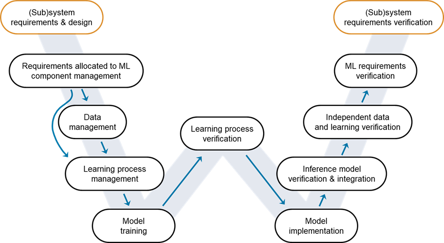
This post is dedicated to learning process verification. We will show you how to ensure that specific verification techniques are in place to guarantee that the pneumonia detection model trained in the previous blog post meets the identified model requirements.

Figure 1: W-shaped development process, highlighting the stage covered in this post. Credit: EASA, Daedalean.

 

Testing and Understanding Model Performance

The model was trained using fast gradient sign method (FGSM) adversarial training, which is a method for training networks so that they are robust to adversarial examples. After training the model, particularly following adversarial training, it is crucial to assess its accuracy using an independent test set.

The model we developed achieved an accuracy exceeding 90%, which not only meets our predefined requirement but also surpasses the benchmarks reported in the foundational research for comparable neural networks. To gain a more nuanced understanding of the model’s performance, we examine the confusion matrix, which sheds light on the types of errors the model makes.

Figure 2: Confusion chart for the adversarially-trained model.

Explainability techniques like Grad-CAM offer a visual understanding of the influential regions in the input image that drive the model’s predictions, enhancing interpretability and trust in the AI model’s decision-making process. Grad-CAM highlights the regions of the input image that contributed most to the final prediction.

Figure 3: Understanding network predictions using Gradient-weighted Class Activation Mapping (Grad-CAM).

 

Verify Robustness of Deep Learning Models

Adversarial Examples

Robustness of the AI model is one of the main concerns when deploying neural networks in safety-critical situations. It has been shown that neural networks can misclassify inputs due to small imperceptible changes.

Consider the case of an X-ray image that a model correctly identifies as indicative of pneumonia. When a subtle perturbation is applied to this image (that is, a small change is applied to each pixel of the image), the model’s output shifts, erroneously classifying the X-ray as normal.

Figure 4: Adversarial examples: effect of input perturbation to image classification.

 

L-infinity norm

To understand and quantify these perturbations, we turn to the concept of the l-infinity norm.

Imagine you have a chest X-ray image. A perturbation with an l-infinity norm of, say, 5 means adding or subtracting any number from 0 to 5 to any number of pixels. In one scenario, you might add 5 to every pixel within a specific image region. Alternatively, you could adjust various pixels by different values within the range of -5 to 5 or alter just a single pixel.

Figure 5: L-infinity norm: examples of possible input perturbations.

However, the challenge is that we need to account for all possible combinations of perturbations within the -5 to 5 range, which essentially presents us with an infinite number of scenarios to test. To navigate this complexity, we employ formal verification methods, which provide a systematic approach to testing and ensuring the robustness of our neural network against a vast landscape of potential adversarial examples.

Formal verification

Given one of the images in the test set, we can choose a perturbation that defines a collection of perturbed images for this specific image. It is important to note that this collection of images is extremely large (the images depicted in the volume in Figure 5 are just a representative sample), and it is not practical to test each perturbed image individually.

Deep Learning Toolbox Verification Library allows you to verify and test robustness of deep learning networks using formal verification methods, such as abstract interpretation. The library enables you to verify whether the network you have trained is adversarially robust with respect to the class label provided an input perturbation.

Figure 6: Formal verification using abstract interpretation.

Formal verification methods offer a mathematical approach that may be used to have formal proof of the correctness of a system. It allows us to conduct rigorous tests across the entire volume of perturbed images to see if the network’s output is affected. There are three potential outcomes for each of the images:

• Verified - The output label remains consistent.
• Violated - The output label changes.
• Unproven - Further verification efforts or model improvement is needed.

Let’s set up the perturbation for our specific problem. The image values in our test set (XTest) range from 0 to 1. We set the perturbation to 1%, up or down. We set the perturbation bounds by using XLower and XUpper and define a collection of images (i.e., the volume in Figure 5). This means that we will test all possible perturbations of images that fall within these bounds.

Before running the verification test, we must convert the data to a dlarray object. The data format for the dlarray object must have the dimensions “SSCB” (spatial, spatial, channel, batch) to represent 2-D image inputs. Note that XTest is not just a single image but a batch of images to verify. So, we have a volume to verify for each of the images in the test set.

perturbation = 0.01; 
XLower = XTest - perturbation; 
XUpper = XTest + perturbation; 
XLower = dlarray(XLower,"SSCB"); 
XUpper = dlarray(XUpper,"SSCB"); 

We are now ready to use the verifyNetworkRobustness function. We specify the trained network, the lower and upper bounds, and the ground truth labels for the images.

result = verifyNetworkRobustness(net,XLower,XUpper,TTest); 
summary(result) 

verified 402

violated 13

unproven 209

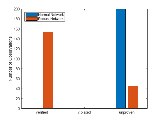
The outcome reveals over 400 images verified, 13 violations, and more than 200 unproven results. We’ll have to go back to those images where the robustness test returned violated or unproven results and see if there is anything we can learn. But for over 400 images, we were able to formally prove that no adversarial example within a 1% perturbation range alters the network’s output—and that’s a significant assurance of robustness.

Another question that we can answer with formal verification is if adversarial training contributed to network robustness. In the second post of the series, we began with a reference model and investigated various training techniques, ultimately adopting an adversarially trained model. Had we used the original network, we would have faced unproven results for nearly all images. And in a safety-critical context, you’ll likely need to treat the unproven results as violations. While data augmentation contributed to verification success, adversarial training enabled the verification of substantially more images, leading to a superiorly robust network that satisfies our robustness requirements.

Figure 7: Comparing verification results from various trained networks.

 

Out-of-Distribution Detection

A trustworthy AI system should produce accurate predictions in a known context. Still, it should also be able to identify unknown examples to the model and reject them or defer them to a human expert for safe handling. Deep Learning Toolbox Verification Library also includes functionality for out-of-distribution (OOD) detection.

Consider a sample image from our test set. To evaluate the model’s ability to handle OOD data, we can derive new test sets by applying meaningful transformations to the original images, as shown in the following figure.

Figure 8: Derived datasets to explore out-of-distribution detection.

Using this library, you can create an out-of-distribution data discriminator to assign confidence to network predictions by computing a distribution confidence score for each observation. It also provides a threshold for separating the in-distribution from the out-of-distribution data.

In the following chart, we observe the network distribution scores for the training data, represented in blue, which constitutes the in-distribution dataset. We also see scores for the various transformations applied to the test set.

Figure 9: Distribution of confidence scores for the original and derived datasets.

By using the distribution discriminator and the obtained threshold, when the model has to classify images with a transformation at test time, we can tell that if the images would be considered in- or out-of- distribution. For example, the images with speckle noise (see Figure 8), would be in-distribution, so we could trust the network output. On the contrary, the distribution discriminator considers the images with the FlipLR and contrast transformations (also see Figure 8) as out-of-distribution, so we shouldn’t trust the network output in those situations.

 

What’s Next?

Stay tuned for our fourth and final blog post, where we will navigate the right-hand side of the W-diagram, focusing on deploying and integrating our robust pneumonia detection model into its operational environment. We will show how to bridge the gap between a well-trained model and a fully functional AI system that can be trusted in a clinical setting.