
Verification and Validation for AI: From requirements to robust modeling
The following post is from Lucas García, Product Manager for Deep Learning Toolbox.
This is the second post in a 4-post series on Verification and Validation for AI. In the first post, we gave an overview of the importance of Verification and Validation in AI within the context of AI Certification. We also introduced the W-shaped development process, an adaptation of the classical V-cycle to AI applications.
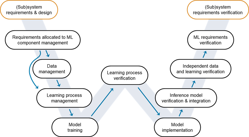 Figure 1: W-shaped development process. Credit: EASA, Daedalean.
This blog post focuses on the steps you need to complete and iterate on starting with collecting requirements and up to creating a robust AI model. To illustrate the verification and validation steps from requirements to modeling, we will use as an example the design of a pneumonia detector.
Figure 1: W-shaped development process. Credit: EASA, Daedalean.
This blog post focuses on the steps you need to complete and iterate on starting with collecting requirements and up to creating a robust AI model. To illustrate the verification and validation steps from requirements to modeling, we will use as an example the design of a pneumonia detector.
Figure 2: MedMNISTv2 dataset – The dataset is licensed under Creative Commons Attribution 4.0 International (CC BY 4.0).
In this post, we’ll address the steps on the left-hand side of the W-cycle to create a Pneumonia Detector using the MedMNIST dataset, starting with Requirements allocated to ML component management all the way down to Model training. However, note that this is not a linear process, particularly when we evaluate the results of the training phase, so we’ll have to iterate to refine our approach.
Figure 3: Requirements Editor: Capturing requirements for the Machine Learning component.
We’ve set a slightly audacious goal with the test precision requirement, aiming to surpass 90% accuracy (the original paper achieved 88% accuracy for similar models). At the same time, we have introduced robustness requirements and other Machine Learning-related requirements we must simultaneously satisfy.
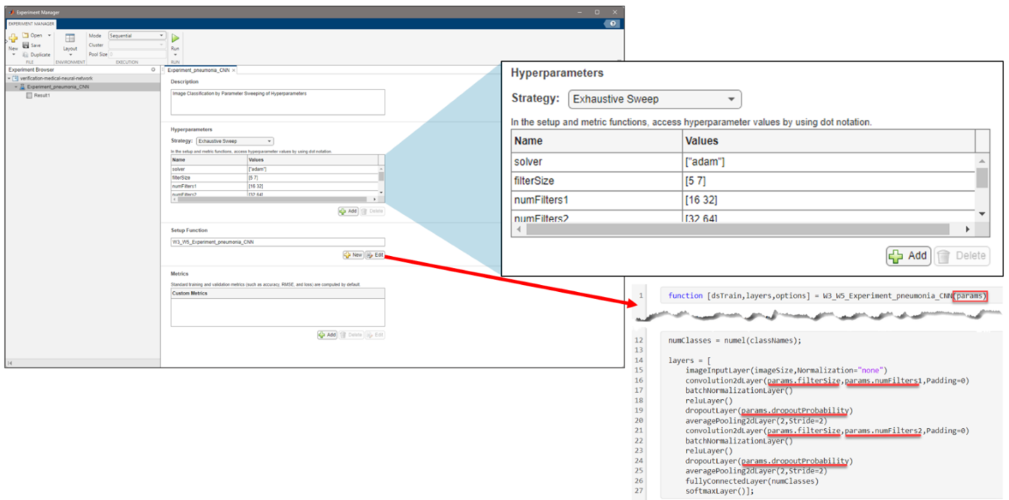 Figure 4: Setting up the problem in Experiment Manager to find an optimal set of hyperparameters from the exported architecture in Deep Network Designer.
Figure 5: Finding an initial model with the Experiment Manager app.
Although we seem to have obtained good results with our model (~96% accuracy for the validation dataset), this model will fail to comply with some of the other requirements we established earlier (e.g., robustness).
We mentioned before that even though the W-cycle seems linear, we often must iterate on our design. To do so, we explored additional training techniques. First, we did data-augmented training, that is, we performed meaningful transformations to the images (rotation, translation, scaling, etc.). This results in better generalization, less overfitting, and improving the model robustness.
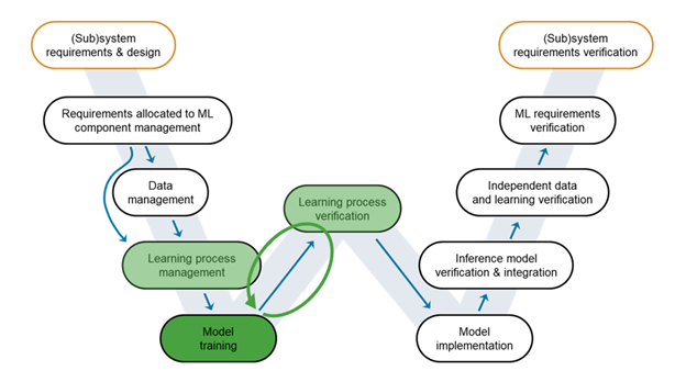 Figure 6: An iterative approach towards building an accurate and robust model.
However, as we’ll see in a future blog post, this data-augmented training will not be enough for our purposes. So, our last iteration will involve using a training algorithm called the Fast Gradient Sign Method (FGSM) for Adversarial Training (learn more). The goal is to generate adversarial examples during training, which are visually similar to the original input data but can cause the model to make incorrect predictions.
Stay tuned for our next blog post. We’ll address the next stage in the W-cycle, the exciting topic of Learning process verification.
Figure 6: An iterative approach towards building an accurate and robust model.
However, as we’ll see in a future blog post, this data-augmented training will not be enough for our purposes. So, our last iteration will involve using a training algorithm called the Fast Gradient Sign Method (FGSM) for Adversarial Training (learn more). The goal is to generate adversarial examples during training, which are visually similar to the original input data but can cause the model to make incorrect predictions.
Stay tuned for our next blog post. We’ll address the next stage in the W-cycle, the exciting topic of Learning process verification.
Figure 1: W-shaped development process. Credit: EASA, Daedalean.
This blog post focuses on the steps you need to complete and iterate on starting with collecting requirements and up to creating a robust AI model. To illustrate the verification and validation steps from requirements to modeling, we will use as an example the design of a pneumonia detector.
Verification and Validation for Pneumonia Detection
Our goal is to verify a deep learning model that identifies whether a patient is suffering from pneumonia by examining chest X-ray images. The image classification model needs to be not only accurate but also highly robust to avoid the potentially severe consequences of a misdiagnosis. We’ll identify the problem and take it through all the steps in the W-shaped development process (W-cycle for short). The dataset we will be using is the MedMNISTv2 dataset. If you are familiar with MNIST for digit classification, MedMNIST is a collection of labeled 2D and 3D biomedical lightweight 28 by 28 images. We decided to use this dataset because of its simplicity and the ability to rapidly iterate over the design. More specifically, we’ll use the PneumoniaMNIST dataset, which is part of the MedMNISTv2 collection.
Requirements Allocated to ML Component Management
We’ll start with the first step in the W-cycle related to AI and Machine Learning; collecting the requirements specific to the Machine Learning component. Note that for any non-Machine Learning component items, you can follow the V-cycle frequently used for development assurance of traditional software. At this stage, key questions to consider are:- Are all the requirements implemented?
- How are the requirements going to be tested?
- Can the model behavior be explained?

Data Management
The next step in the W-cycle is Data management. Since we are solving a supervised learning problem, we need labeled data for training the model. MATLAB offers various labeling apps (including Image Labeler and Signal Labeler) that are extremely useful at this point, allowing you to label your dataset interactively (and with automation). Thankfully, data has already been labeled into “pneumonia” and “normal” images. I would have to seek expert advice to label X-ray images or find the right algorithm to automate the process. The data set has also been partitioned into training, validation, and testing sets. So, we don’t need to worry about that either. All we need to worry about at this point is to conveniently manage our images. The imageDatastore object allows you to manage a collection of image files where each individual image fits in memory, but the entire collection does not necessarily fit. Indeed, the MedMNIST images are small and will all fit in memory, but using a data store allows you to see how you can create a scalable process for more realistic workflows. By indicating the folder structure and that the label source can be inferred from the folder names, we can create a MATLAB object that acts as an image data repository.trainingDataFolder = "pneumoniamnist\Train"; imdsTrain = imageDatastore(trainingDataFolder,IncludeSubfolders=true,LabelSource="foldernames"); countEachLabel(imdsTrain)
ans =

  2×2 table

      Label      Count
    _________    _____

    normal       1214
    pneumonia    3494
Note that the dataset is imbalanced towards more pneumonia samples. So, this should be considered in the loss function as we train the model.
Learning Process Management
At this stage, we’d like to account for all the preparatory work before the training phase. We’ll focus on developing the network architecture and choosing the training options (training algorithm, loss function, hyperparameters, etc.). You can easily design and visualize the network interactively using the Deep Network Designer app. Once you have designed the network (in this case, a simple CNN for image classification), MATLAB code can be generated for training.numClasses = numel(classNames);
layers = [
imageInputLayer(imageSize,Normalization="none")
convolution2dLayer(7,64,Padding=0)
batchNormalizationLayer()
reluLayer()
dropoutLayer(0.5)
averagePooling2dLayer(2,Stride=2)
convolution2dLayer(7,128,Padding=0)
batchNormalizationLayer()
reluLayer()
dropoutLayer(0.5)
averagePooling2dLayer(2,Stride=2)
fullyConnectedLayer(numClasses)
softmaxLayer];
However, coming up with the optimal hyperparameters might not be so straightforward. The Experiment Manager app helps you find the optimal training options for neural networks by sweeping through a range of hyperparameter values or using Bayesian optimization. You can run different training configurations, even in parallel, if you have access to the necessary hardware.
Figure 4: Setting up the problem in Experiment Manager to find an optimal set of hyperparameters from the exported architecture in Deep Network Designer.
Model Training
It is now time to train the model - or more accurately, models. We first run the experiment we have configured in the Experiment Manager app. This gives us an excellent model to start with. Figure 6: An iterative approach towards building an accurate and robust model.
However, as we’ll see in a future blog post, this data-augmented training will not be enough for our purposes. So, our last iteration will involve using a training algorithm called the Fast Gradient Sign Method (FGSM) for Adversarial Training (learn more). The goal is to generate adversarial examples during training, which are visually similar to the original input data but can cause the model to make incorrect predictions.
Stay tuned for our next blog post. We’ll address the next stage in the W-cycle, the exciting topic of Learning process verification.
Figure 6: An iterative approach towards building an accurate and robust model.
However, as we’ll see in a future blog post, this data-augmented training will not be enough for our purposes. So, our last iteration will involve using a training algorithm called the Fast Gradient Sign Method (FGSM) for Adversarial Training (learn more). The goal is to generate adversarial examples during training, which are visually similar to the original input data but can cause the model to make incorrect predictions.
Stay tuned for our next blog post. We’ll address the next stage in the W-cycle, the exciting topic of Learning process verification. 


Comments
To leave a comment, please click here to sign in to your MathWorks Account or create a new one.