
Physics-Informed Machine Learning: Methods and Implementation
This blog post is from Mae Markowski, Senior Product Manager at MathWorks.
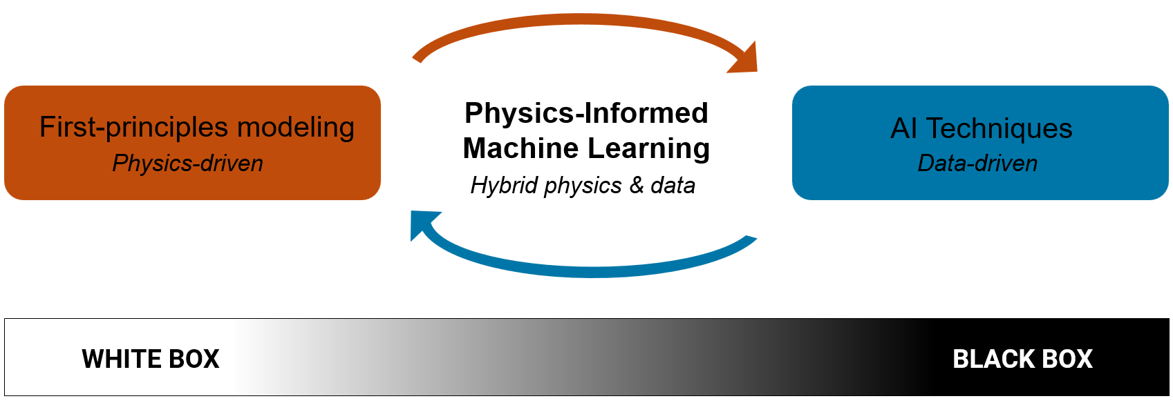
In our previous post, we laid the groundwork for physics-informed machine learning, exploring what it is, why it matters, and how it can be applied across different science and engineering domains. We used a pendulum example to make the concepts discussed more concrete.
In this post, we’ll dive deeper into specific physics-informed machine learning methods, categorized by their primary objectives: modeling complex systems from data, discovering governing equations, and solving known equations.
To illustrate the main ideas behind each method, we will apply them to the familiar pendulum example with accompanying MATLAB code snippets. For the full set of examples featured in this post, see Physics-Informed Machine Learning Methods and Implementation supporting code, and for more advanced examples, check out the Github repository SciML and Physics-Informed Machine Learning Examples.
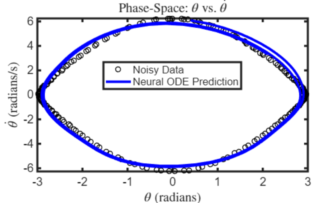 Figure 1: Neural ODE predicts the pendulum’s trajectory from noisy measurement data.
While Neural ODEs model how system states evolve, they don’t account for the variables we want to observe, which are essential for control, estimation, and system identification. Neural state-space models address this by also learning an observation equation that relates states to outputs, which we will explore next.
Figure 1: Neural ODE predicts the pendulum’s trajectory from noisy measurement data.
While Neural ODEs model how system states evolve, they don’t account for the variables we want to observe, which are essential for control, estimation, and system identification. Neural state-space models address this by also learning an observation equation that relates states to outputs, which we will explore next.
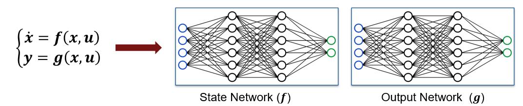 Figure 2: Neural state-space predictions of the system’s state and output. Here, \( x_1 \) and \( x_2 \) represent the angular position and angular velocity, and \( y_1 \) and \( y_2 \) correspond to the horizontal and vertical positions of the pendulum’s point mass, respectively. For the full example, see Neural State-Space Model of Simple Pendulum System.
Consider a pendulum system where the states are angular position and velocity, the input is an applied torque, and the outputs are the horizontal and vertical positions of the mass. You can create a neural state-space model using System Identification Toolbox to learn both the state dynamics and output function of the system directly from data.
Figure 2: Neural state-space predictions of the system’s state and output. Here, \( x_1 \) and \( x_2 \) represent the angular position and angular velocity, and \( y_1 \) and \( y_2 \) correspond to the horizontal and vertical positions of the pendulum’s point mass, respectively. For the full example, see Neural State-Space Model of Simple Pendulum System.
Consider a pendulum system where the states are angular position and velocity, the input is an applied torque, and the outputs are the horizontal and vertical positions of the mass. You can create a neural state-space model using System Identification Toolbox to learn both the state dynamics and output function of the system directly from data.
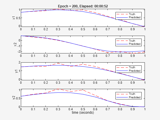 Figure 3: Neural state-space predictions of the state (angular position and velocity) and output (horizontal and vertical positions of point mass). For the full example, see Neural State-Space Model of Simple Pendulum System.
Neural state-space models are especially useful in controls, estimation, optimization, and reduced order modeling. However, neural state-space models, like neural ODEs, treat the system’s dynamics as entirely unknown even when parts of the dynamics are well known, a limitation that is addressed by Universal Differential Equations.
Figure 3: Neural state-space predictions of the state (angular position and velocity) and output (horizontal and vertical positions of point mass). For the full example, see Neural State-Space Model of Simple Pendulum System.
Neural state-space models are especially useful in controls, estimation, optimization, and reduced order modeling. However, neural state-space models, like neural ODEs, treat the system’s dynamics as entirely unknown even when parts of the dynamics are well known, a limitation that is addressed by Universal Differential Equations.
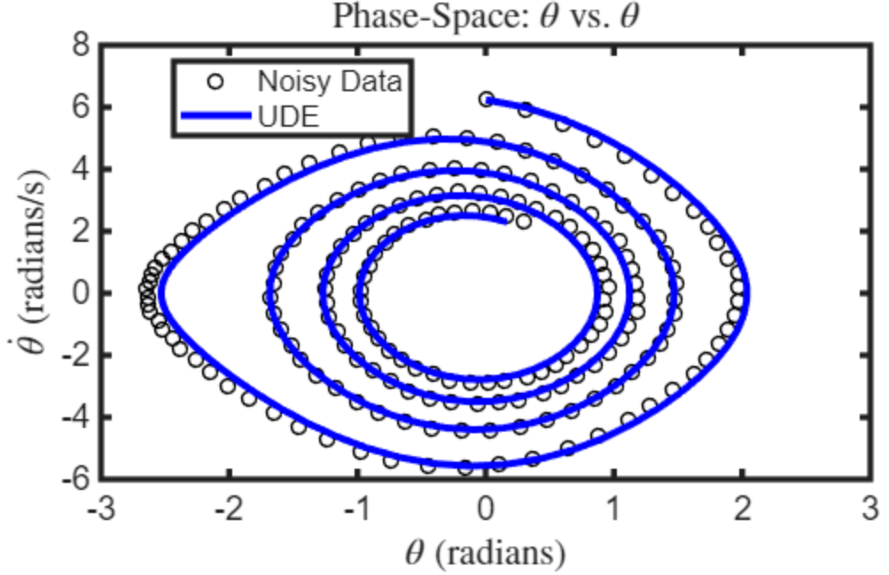 Figure 4: UDEs model the unknown damping force of the pendulum to predict its trajectory from data.
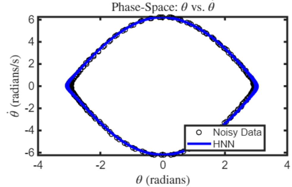 Figure 5: HNNs predict the pendulum’s trajectory and are designed to conserve energy.
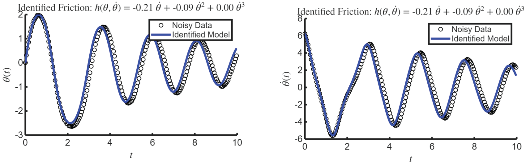 Figure 6: Here SINDy is used to identify a mechanistic form for the friction from pendulum trajectory data.
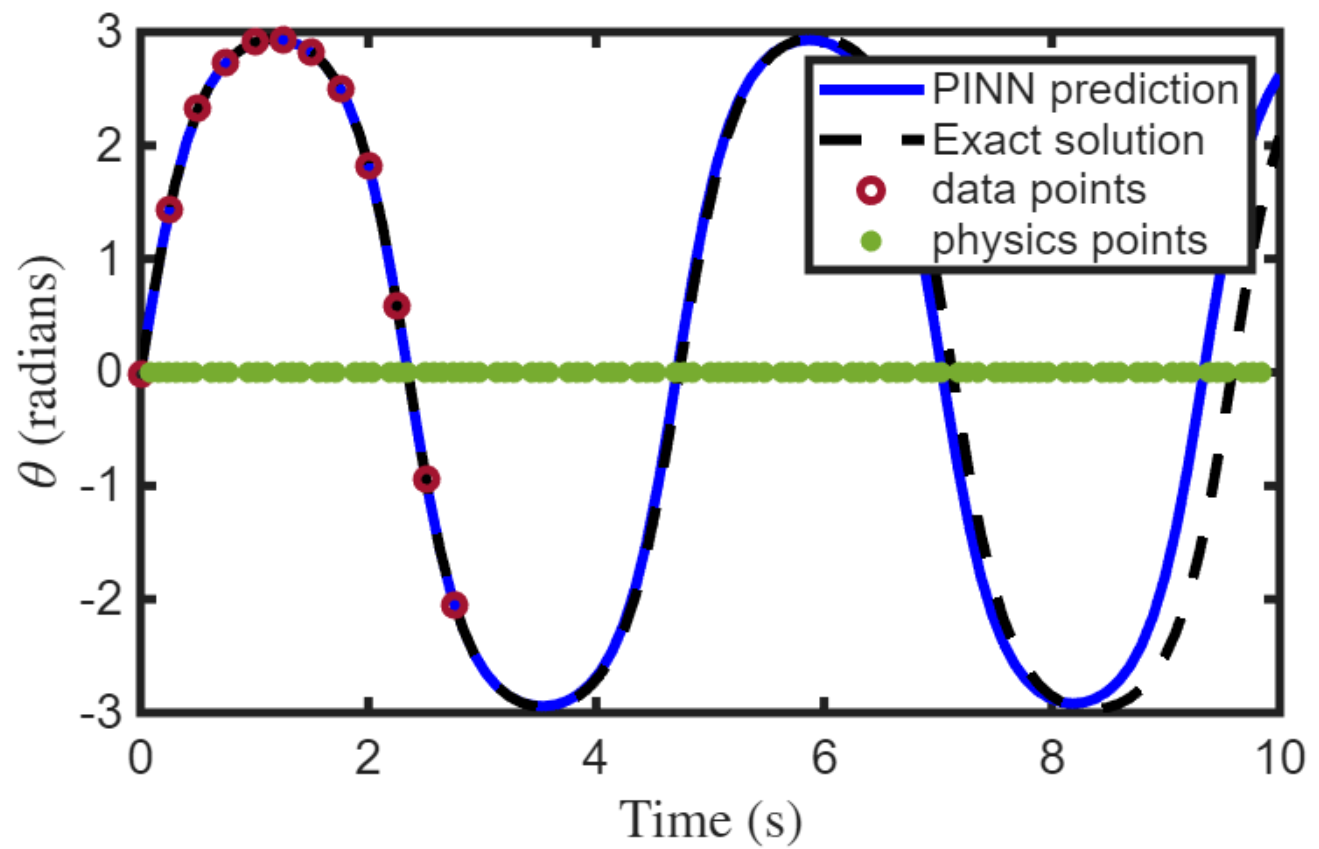 Figure 7: PINN predicts the angle over time using the governing pendulum equation and observations of the pendulum’s angle.
While PINNs may not outperform traditional numerical methods for simple, low-dimensional problems like the pendulum, they can provide advantages for high-dimensional partial differential equations (PDEs), inverse problems, and cases with a blend of data and physical equations.
Figure 7: PINN predicts the angle over time using the governing pendulum equation and observations of the pendulum’s angle.
While PINNs may not outperform traditional numerical methods for simple, low-dimensional problems like the pendulum, they can provide advantages for high-dimensional partial differential equations (PDEs), inverse problems, and cases with a blend of data and physical equations.
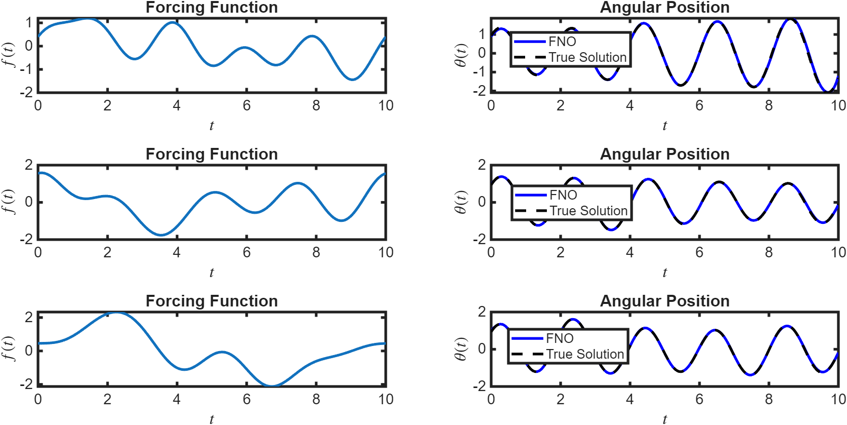 Figure 8: Fourier Neural Operator learns mappings between function spaces, such as the map from forcing function to angular position in the pendulum example.
While a neural operator is not necessary for simple problems like the pendulum, since re-solving the pendulum equation for a new \(f\) is computationally inexpensive, they are especially useful for repeated large-scale PDE simulations where traditional solvers can require substantial computation time.
Figure 8: Fourier Neural Operator learns mappings between function spaces, such as the map from forcing function to angular position in the pendulum example.
While a neural operator is not necessary for simple problems like the pendulum, since re-solving the pendulum equation for a new \(f\) is computationally inexpensive, they are especially useful for repeated large-scale PDE simulations where traditional solvers can require substantial computation time.
Table 1: Summary of physics-informed machine learning approaches for modeling unknown dynamics, identifying governing equations, and solving known PDEs and ODEs. The “Physics Embedded?” column indicates the degree to which physical knowledge is incorporated: a circle denotes a weak embedding (e.g., physics-inspired architecture), while a checkmark indicates direct and explicit use of physics in the model objective, structure or loss. The “Notes” column highlights typical contexts where each approach is particularly suitable.
Modeling Unknown Dynamics from Data
Neural Ordinary Differential Equation
When modeling physical systems like a pendulum, we often use differential equations of the form: \[\dot{x} = f(x, u) ,\] where \(x \) represents the state (like the pendulum’s angular position and velocity), \(u \) represents any external inputs, and \(f \) represents the system’s dynamics. However, in many scenarios, the dynamics function \(f \) is either unknown or is too complex to describe analytically. Neural Ordinary Differential Equations (Neural ODEs) address this challenge by using a neural network to learn \(f \) directly from data. This makes neural ODEs a powerful tool for modeling systems with unknown dynamics, especially when working with time-series data that is irregularly sampled. While neural ODEs do not embed known physical laws directly into the model, they can be generalized to incorporate partially known dynamics, such as in Universal Differential Equations, which we’ll discuss later in the post. For example, suppose you have measurements of a pendulum’s angular position and velocity but lack the explicit governing equations. You can train a neural ODE to learn the pendulum dynamics from the given trajectory data. Below is a code snippet illustrating how to set up a neural ODE using Deep Learning Toolbox.% Model unknown dynamics f(x) using multilayer perceptron (MLP)
fLayers = [
featureInputLayer(2, Name="input")
fullyConnectedLayer(32)
geluLayer
fullyConnectedLayer(32)
geluLayer
fullyConnectedLayer(2, Name="output")];
fNet = dlnetwork(fLayers);
% Construct a neural ODE using neuralODElayer to solve ODE system for x
nODElayers = [
featureInputLayer(2, Name="IC_in")
neuralODELayer(fNet, tTrain, ...
GradientMode="adjoint", ...
Name="ODElayer")];
nODEnet = dlnetwork(nODElayers);
This code defines the neural network fnet to represent the unknown pendulum dynamics, then uses a neuralODELayer to solve the ODE system \(\dot{x} = f(x) \), where the righthand side is given by the output of fNet. Once trained, the model predicts the system’s states over a specified time interval by numerically integrating the ODE forward in time from a given initial state, using an ODE solver like ode45.
Figure 1: Neural ODE predicts the pendulum’s trajectory from noisy measurement data.
While Neural ODEs model how system states evolve, they don’t account for the variables we want to observe, which are essential for control, estimation, and system identification. Neural state-space models address this by also learning an observation equation that relates states to outputs, which we will explore next.
Neural State-Space
Neural State-Space models extend neural ODEs by incorporating a state-space structure: \[\dot{x} = f(x, u), \quad y = g(x, u) ,\] where the state dynamics function \(f\) and the output function \(g\) are each modeled using neural networks.
Figure 2: Neural state-space predictions of the system’s state and output. Here, \( x_1 \) and \( x_2 \) represent the angular position and angular velocity, and \( y_1 \) and \( y_2 \) correspond to the horizontal and vertical positions of the pendulum’s point mass, respectively. For the full example, see Neural State-Space Model of Simple Pendulum System.
Consider a pendulum system where the states are angular position and velocity, the input is an applied torque, and the outputs are the horizontal and vertical positions of the mass. You can create a neural state-space model using System Identification Toolbox to learn both the state dynamics and output function of the system directly from data.
% Create neural state-space model with 2 states, 1 input, 4 outputs
sys = idNeuralStateSpace(2,NumInputs=1,NumOutput=4);

% State network
sys.StateNetwork = createMLPNetwork(sys,'state', ...
   LayerSizes=[128 128], ...
   Activations="tanh");

% Output network
sys.OutputNetwork(2) = createMLPNetwork(sys,'output', ...
   LayerSizes=[128 128], ...
   Activations="tanh");
Figure 3: Neural state-space predictions of the state (angular position and velocity) and output (horizontal and vertical positions of point mass). For the full example, see Neural State-Space Model of Simple Pendulum System.
Neural state-space models are especially useful in controls, estimation, optimization, and reduced order modeling. However, neural state-space models, like neural ODEs, treat the system’s dynamics as entirely unknown even when parts of the dynamics are well known, a limitation that is addressed by Universal Differential Equations.
Universal Differential Equation
For some systems, part of the dynamics may be well understood, while other effects are difficult to capture with traditional physics-based models. In such cases, Universal Differential Equations (UDEs) offer a hybrid approach that combines known physics with machine-learned components. For the pendulum, you might know the main dynamics (e.g. angular acceleration \( \ddot{\theta} \) and restoring force \( -\omega_0^2 \sin \theta \)) but suspect there is unmodeled friction. You can write the system as: \[ \frac{d}{dt} \begin{bmatrix} \theta \\ \dot{\theta} \end{bmatrix} = \begin{bmatrix} \dot{\theta} \\ - \omega_0^2 \sin \theta + h(\theta, \dot{\theta}) \end{bmatrix} = g(\theta, \dot{\theta}) + \begin{bmatrix} 0 \\ h(\theta, \dot{\theta}) \end{bmatrix}, \] where \(g\) represents the known dynamics and \(h \) represents the unknown friction force, which is learned from data using a neural network. With Deep Learning Toolbox, you can implement a UDE for this problem by defining the known physics with a functionLayer, modeling the unknown friction with a neural network, combining them into a single network, and then wrapping in a neuralODElayer to solve the full system.% Define the known physics in functionLayer
gFcn = @(X) [X(2,:); -omega0^2*sin(X(1,:))];
gLayer = functionLayer(gFcn, Acceleratable=true, Name="g");
% Model unknown friction force using a multilayer perceptron (MLP)
hLayers = [
fullyConnectedLayer(16,Name="fc1")
geluLayer
fullyConnectedLayer(1,Name="h")];
% Combine known and unknown components
combineFcn = @(x, y) [x(1,:); x(2,:) + y];
combineLayer = functionLayer(combineFcn,Name="combine",Acceleratable=true);
fNet = [featureInputLayer(2,Name="input")
gLayer
combineLayer];
fNet = dlnetwork(fNet,Initialize=false);
fNet = addLayers(fNet,hLayers);
fNet = connectLayers(fNet,"input","fc1");
fNet = connectLayers(fNet,"h","combine/in2");
% Wrap in neuralODELayer
nODElayers = [
featureInputLayer(2, Name="IC_in")
neuralODELayer(fNet, tTrain, ...
GradientMode="adjoint", ...
Name="ODElayer")];
nODEnet = dlnetwork(nODElayers);
Figure 4: UDEs model the unknown damping force of the pendulum to predict its trajectory from data.
Hamiltonian Neural Network
Unlike the previous methods we discussed which learn the system’s state evolution directly, Hamiltonian Neural Networks (HNNs) learn the Hamiltonian \(H \), a function that represents the system’s total energy in terms of position \( q \) and momentum \( p \). Once trained, the system state is recovered by applying Hamilton’s equations to the learned Hamiltonian: \[ \dot{q} = \frac{\partial H}{\partial p}, \quad \dot{p} = -\frac{\partial H}{\partial q}. \] This added structure makes HNNs well-suited for modeling systems where total energy is conserved, like the undamped pendulum. To train the model, a custom loss function penalizes the difference between the observed values of \( \dot{q} \) and \( \dot{p} \) and the corresponding partial derivatives of the network, computed using automatic differentiation. The code snippet below constructs a network to learn the Hamiltonian from the undamped pendulum trajectory data, defines a custom loss function based on Hamilton’s equations, and shows how to make predictions with the trained network using an ODE solver like ode45.% Define a neural network to learn the Hamiltonian function H(q,p)
fcBlock = [
fullyConnectedLayer(64)
tanhLayer];
layers = [
featureInputLayer(2)
repmat(fcBlock,[2 1])
fullyConnectedLayer(1)];
net = dlnetwork(layers);
net = dlupdate(@double, net);
% Define custom loss function to penalize deviations from Hamilton’s equations
function [loss,gradients] = modelLoss(net, qp, qpdotTarget)
qpdot = model(net, qp);
loss = l2loss(qpdot, qpdotTarget, DataFormat="CB");
gradients = dlgradient(loss,net.Learnables);
end
function qpdot = model(net, qp)
H = forward(net,dlarray(qp,'CB'));
H = stripdims(H);
qp = stripdims(qp);
dH = dljacobian(H,qp,1);
qpdot = [dH(2,:); -1.*dH(1,:)];
end
% Enforce Hamiltonian structure by solving Hamilton’s equations with learned H
accModel = dlaccelerate(@model);
tspan = tTrain;
x0 = dlarray([q(1); p(1)]); % initial conditions
odeFcn = @(ts,xs) dlfeval(accModel, net, xs);
[~, qp] = ode45(odeFcn, tspan, x0);
qp = qp'; % Transpose to return to (2)x(N)
Figure 5: HNNs predict the pendulum’s trajectory and are designed to conserve energy.
Discovering Equations
Sparse Identification of Nonlinear Dynamics
While the methods we’ve discussed so far are effective at capturing system behavior, they don’t necessarily yield interpretable models. In some applications, like quantitative systems pharmacology, understanding the dynamics can be just as important as learning them. In these cases, equation discovery techniques like Sparse Identification of Nonlinear Dynamics (SINDy) offer a way to extract mathematical models describing the dynamics directly from data. SINDy assumes that the system’s dynamics can be expressed as a sparse linear combination of candidate functions, such as polynomials and trigonometric functions, and identifies the most relevant terms using sparse regression. This results in a compact, interpretable model that captures the underlying physics. For example, in the case of the damped pendulum, we can combine the previously described UDE approach with SINDy to recover a mechanistic form for the friction force. In this example, the true friction term is \[ h(\theta, \dot{\theta}) = -(c_1 + c_2 \dot{\theta}) \dot{\theta}, \] where \(c_1=0.2\) and \(c_2= 0.1\). The following code extracts the learned friction term from the UDE and uses SINDy to uncover a mathematical model that describes it.% Extract trained network representing the learned friction from the UDE
fNetTrained = nODEnet.Layers(2).Network;
hNetTrained = removeLayers(fNetTrained,["g","combine"]);
lrn = hNetTrained.Learnables;
lrn = dlupdate(@dlarray, lrn);
hNetTrained = initialize(hNetTrained);
hNetTrained.Learnables = lrn;
% Evaluate the learned friction term at the training data points
hEval = predict(hNetTrained,Y',InputDataFormats="CB");
% Define candidate basis functions for SINDy: omega, omega^2, omega^3
e1 = @(X) X(2,:);
e2 = @(X) X(2,:).^2;
e3 = @(X) X(2,:).^3;
E = @(X) [e1(X); e2(X); e3(X)];
% Evaluate the basis functions at the training points
EEval = E(Y');
% Sequentially solve h = W*E with thresholding to induce sparsity
iters = 10;
threshold = 0.05;
Ws = cell(iters,1);
% Initial least-squares solution for W
W = hEval/EEval;
Ws{1} = W;
for iter = 2:iters
% Zero out small coefficients for sparsity
belowThreshold = abs(W)<threshold;
W(belowThreshold) = 0;
% Recompute nonzero coefficients using least squares
for i = 1:size(W,1)
aboveThreshold_i = ~belowThreshold(i,:);
W(i,aboveThreshold_i) = hEval(i,:)/EEval(aboveThreshold_i,:);
end
Ws{iter} = W;
end
% Display the identified equation for the friction term
Widentified = Ws{end};
fprintf(...
"Identified h = %.2f y + %.2f y^2 + %.2f y^3 \n", ...
Widentified(1), Widentified(2), Widentified(3))
Figure 6: Here SINDy is used to identify a mechanistic form for the friction from pendulum trajectory data.
Solving Known Equations
Physics-Informed Neural Network
So far, we’ve looked at methods that learn the system’s dynamics. Rather than learning the dynamics themselves, Physics-Informed Neural Networks (PINNs) learn the solution to a known differential equation by embedding this equation directly into the loss function. This is typically achieved using automatic differentiation or other numerical differentiation techniques. PINNs incorporate the governing equations as soft constraints in the loss function, penalizing deviations from the physical laws during training. They can also easily incorporate available measurement data of the solution function into the loss function as an additional, supervised term. For the pendulum, you can use Deep Learning Toolbox to define a custom loss function that penalizes deviations from the governing equation \(\ddot{\theta} = -\omega_0^2 \sin \theta \) :function loss = physicsInformedLoss(net,T,omega_0) Theta = forward(net,T); Thetatt = dllaplacian(stripdims(Theta),stripdims(T),1); residual = Thetatt + omega0^2*sin(Theta); loss = mean(residual.^2 ,'all'); endFunctions like dljacobian and dllaplacian make it straightforward to compute the derivative terms needed for PINNs. Alternatively, you can generate a PINN loss function directly from a symbolic differential equation using the functionality in PINN Loss Function Generation with Symbolic Math, available for download on File Exchange. The code snippet below provides an example usage of this functionality for the same pendulum equation:
syms theta(t)
pendulumODE = diff(theta,t,t) – omega0^2*sin(theta(t)) == 0;
physicsInformedLoss = ode2PinnLossFunction(pendulumODE,ComputeMeanSquaredError=true);
Figure 7: PINN predicts the angle over time using the governing pendulum equation and observations of the pendulum’s angle.
While PINNs may not outperform traditional numerical methods for simple, low-dimensional problems like the pendulum, they can provide advantages for high-dimensional partial differential equations (PDEs), inverse problems, and cases with a blend of data and physical equations.
Neural Operator
Neural operators, such as the Fourier Neural Operator (FNO), are a class of neural PDE solvers designed to learn mappings between function spaces. Unlike PINNs, which are typically trained to solve a specific instance of an ODE or PDE, neural operators learn a mapping from the space of input functions (such as initial conditions or forcing functions) directly to the space of solution functions, enabling fast prediction for new scenarios without the need for retraining. Although neural operators do not inherently encode physical laws, their architectures are inspired by the mathematical structure of PDEs. When the governing equations are known, neural operators can be combined with the PINN methodology by embedding those equations into the loss function, resulting in physics-informed neural operators. For example, consider a pendulum which is subject to a time-dependent forcing function , so that \[\ddot{\theta} + \omega_0^2 \sin \theta = f(t) .\] A neural operator can be applied to learn the map from the space of forcing functions to the corresponding space of solution functions. Once trained, the model can rapidly predict the pendulum’s response to new forcing functions. Fourier Neural Operators can be implemented in MATLAB by defining a custom layer in Deep Learning Toolbox, as shown in the documentation example Solve PDE Using Fourier Neural Operator.
Figure 8: Fourier Neural Operator learns mappings between function spaces, such as the map from forcing function to angular position in the pendulum example.
While a neural operator is not necessary for simple problems like the pendulum, since re-solving the pendulum equation for a new \(f\) is computationally inexpensive, they are especially useful for repeated large-scale PDE simulations where traditional solvers can require substantial computation time.
GNN for Geometric Deep Learning
While the FNO is well-suited for problems defined on regular grids, many engineering applications involve data on complex or irregular geometries. In these cases, Graph Neural Networks (GNNs) can provide a powerful alternative by operating directly on mesh or graph-based representations. This makes GNNs particularly effective for large-scale PDE simulations on complex domains. While GNNs may not be relevant for this simple 1D pendulum example, they become valuable tools for more complex domains, such as predicting displacement fields in a robotic arm for different geometric designs. Once trained, GNNs can deliver rapid predictions for new designs, enabling real-time exploration of “what-if” scenarios. To learn how to train a GNN on finite element analysis data for PDE simulations, see the example Solve Heat Equation Using Graph Neural Network.Summary of Methods
See the following summary table for a quick reference of all the physics-informed machine learning methods we discussed throughout this post.| Objective | Approach | What’s Learned? | Physics Embedded? | How is Physics Embedded? | Example Systems | Notes |
| Modeling unknown dynamics | Neural ODE | Dynamics function \(f\) | Architecture: ODE structure | Any ODE system | Flexible for any ODE; handles irregularly sampled time-series data | |
|---|---|---|---|---|---|---|
| Neural State-Space | State-update/output functions | Architecture: ODE & state-space structure | Any ODE system with observable outputs | Can be continuous and discrete; handles irregular sampling if continuous | ||
| UDE | Unknown part of dynamics function | Objective: blends physics with learned corrections; Architecture: ODE structure | ODE systems with partially known dynamics | Leverages partial physics; handles irregular sampling | ||
| HNN | Hamiltonian \(H\) | Loss: Hamilton’s equations encoded as soft constraints; Architecture: Network predicts Hamiltonian \(H \) | Mechanical | Accounts for conservation of energy through model structure | ||
| Discovering equations | SINDy | Sparse coefficients (equations) | Architecture: Sparse regression over function library | Any measurable system | Produces interpretable models | |
| Solving known equations | PINN | Solution to governing equation | Loss: PDE/ODE residuals | Mass-spring, Navier-Stokes | Requires explicit equations; particularly suited for limited data, inverse problems, high-dimensional PDEs | |
| FNO | Solution operator | Architecture: Motivated by spectral methods for PDEs | PDE families, fluid, wave equations | Operates on uniform grids; capable of generalizing across grid resolutions; enables fast what-if analysis after training | ||
| GNN | Solution on irregular geometries | Architecture: Message-passing on graph/mesh | Heat transfer, structural mechanics, CFD on mesh data | Well-suited for complex, irregular geometries; enables fast what-if analysis after training |
Conclusion and Final Thoughts
Throughout this two-part blog series, we have surveyed different scientific and engineering tasks suited to physics-informed machine learning, the types of physics knowledge that can be incorporated, how this knowledge is embedded, and provided educational MATLAB examples along the way. Together, these posts have shown how physics-informed machine learning bridges the gap between data-driven modeling and established scientific principles, and can help with more accurate, reliable, and interpretable predictions. Whether you are just starting to explore this area or looking to implement advanced techniques in your own work, I hope this series has provided you with a solid foundation and practical guidance on the ever-evolving field of physics-informed machine learning. Stay tuned for future posts, and let us know in the comments if there are any topics or techniques that you’d like to learn more about!


댓글
댓글을 남기려면 링크 를 클릭하여 MathWorks 계정에 로그인하거나 계정을 새로 만드십시오.