The following post is from Jue Liu  from Columbia University and Yuchen Dong from MathWorks.

The example featured in the blog can be found on GitHub here.

View the Physics-Informed Neural Networks for Option Pricing by Yuchen Dong from the 2024 MathWorks Finance Conference here:

Option Pricing and the Black-Scholes Model

The Black-Scholes equation is a widely used mathematical model for pricing options and other financial derivatives. It describes the price evolution of an option over time, considering factors such as the underlying asset price, volatility, risk-free interest rate, and the option’s strike price and maturity.

The Black-Scholes equation is a partial differential equation (PDE) of the form:

where  is the price of the option as a function of stock price  and time ,  is the risk-free interest rate, and  is the volatility of the stock returns.

The Black-Scholes equation has an analytical solution, known as the Black-Scholes formula, which gives the exact option price under certain assumptions. However, real-world conditions often deviate from these assumptions, making traditional closed-form solutions inadequate. In such complex or non-ideal scenarios, numerical methods (e.g., finite difference, finite element methods) are often employed, but they may become challenging or computationally expensive.

What are Physics-Informed Neural Networks (PINNs)?

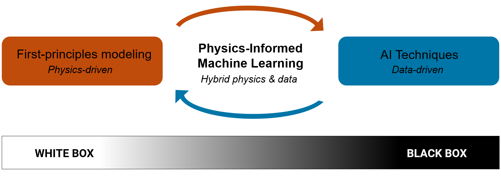
Physics-Informed Neural Networks (PINNs) are a class of deep learning models that incorporate physical laws and domain knowledge into the neural network training process. PINNs are particularly useful for solving PDEs and other physical systems, as they can learn the solution while respecting the underlying governing equations.

PINNs are particularly useful for problems where analytical solutions are difficult or traditional numerical methods may struggle, including scenarios such as:

• Approximating solutions to complex PDEs and ODEs in physics, engineering, and finance.
• Addressing inverse problems where model parameters must be estimated from sparse or limited data, making them valuable when complete measurements are unavailable.

In contrast to traditional purely data-driven models, PINNs integrate these physical or financial-mathematical constraints (such as the Black-Scholes PDE in option pricing) into the loss function. This loss typically includes:

• The PDE residual term, ensuring the network’s predictions satisfy the governing equation.
• The mismatch term between the network’s predictions and the imposed initial and boundary conditions.

By minimizing this composite loss function, the neural network learns to approximate the solution to the PDE while adhering to the physical constraints. As a result, PINNs can handle unknown parameters, ill-posed problems, and scenarios with sparse or noisy data. They also do not rely on predefined computational meshes, which makes them suitable for high-dimensional PDE problems.

Using MATLAB’s Deep Learning Toolbox, we can construct and train PINNs, enabling rapid predictive analysis. PINNs can be seamlessly integrated with MATLAB.

Solving the Black-Scholes Equation with PINNs

In this example, we demonstrate how to solve the Black-Scholes equation using PINNs in MATLAB. The main steps involved are:

1. Generate training data: We create a set of input points (stock prices and times) and corresponding initial and boundary conditions based on the Black-Scholes formula.

We consider a European call option with strike price: , interest rate , volatility , time to maturity  year. We define the domain such that the stock price and . At , we impose the terminal condition: .
Identify and sample points in the  domain for:

• Collocation Points (PDE Residual): Randomly sampled points in the domain where the PDE residual will be enforced.
• Boundary Points: Points corresponding to the boundary conditions, such as and .
• Expiration Points: Points at the terminal time where we apply the payoff condition .

Below is the plot on sampling data points in the selected domain. The plotted figure shows the distribution of collocation points, boundary points, and expiration points throughout the domain, providing a clear overview of where the PINN will learn the solution.

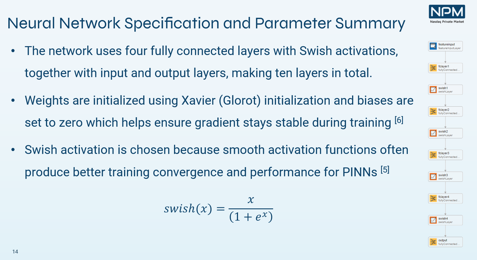
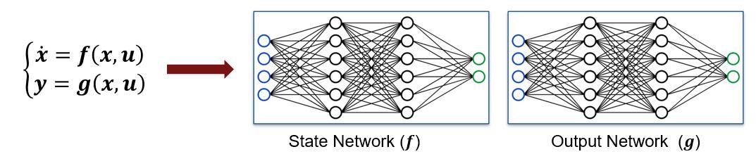
2. Define the neural network architecture: We construct a fully connected neural network with a suitable number of layers and neurons to represent the option price function.

We can visualize and change the settings from Deep Network Designer. In this app, you easily build deep learning networks interactively. Analyze the neural networks to check if the defined architecture is correct and detect problems before training.

3. Customize the loss function: We implement a customized loss function that includes the mismatch between the neural network predictions and the initial and boundary conditions, as well as the residual of the Black-Scholes equation.

The loss function is derived from Black-Scholes PDE. We implement autodifferentiation here to generate the derivative terms in PDE. Autodifferentiation is a widely used tool for deep learning. It is particularly useful for creating and training complex deep learning models without needing to compute derivatives manually for optimization. More information on autodifferentiation in MATLAB can be found here.

4. Train the neural network: We use the Adam optimizer algorithm to minimize the loss function and learn the optimal network parameters.

For training process, we set the number epoch is , and initial learning rate is . You can also use the Experiment Manager for the hyperparameter tuning.

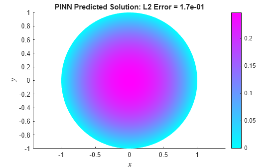
5. Evaluate the trained model: We compare the neural network predictions with the analytical solutions to validate accuracy.

In this section, we compare the numerical solutions with the analytic solutions to Black Scholes PDE at different maturity time .

Comparing the prediction and analytical solutions, the PINNs approximation has the accuracy in the shape of the true solutions. However, the PINNs perform underestimates from the analytic solutions as the maturity time T increases. The accuracy could be improved by considering different types of loss functions. In the current settings, the total loss function is consisted by three components: PDE loss, initial value loss, and boundary value loss. The results may be improved by trying smooth  loss. Another way is to try different neural networks. The activation layers used in the current settings are ReLU Activations. Recommend testing wider networks over deeper ones, utilizing tanh activation function [4].

Conclusion

We have illustrated how to apply PINNs to the Black-Scholes equation, demonstrating a flexible and potentially robust approach to option pricing. While initial results are promising, further refinements in model architecture, training strategies, and loss function design may lead to substantial improvements in accuracy and applicability to a wide range of financial instruments.

Acknowledgments

I extend my sincere gratitude to our mentor, Yuchen Dong, for his patient guidance, valuable insights, and unwavering support throughout this project. His help was instrumental in overcoming challenges and improving our understanding. We would like to thank Ben Wells-Day on reviewing our code. To access our code, please visit our GitHub repository.

Reference

1. Solve Partial Differential Equation with L-BFGS Method and Deep Learning
2. Solve Poisson Equation on Unit Disk Using Physics-Informed Neural Network
3. Dhiman, Y. Hu, Physics Informed Neural Network for Option Pricing, arXiv:2312.06711
4. Wang, S. Sanharan, H. Wang, and P. Perdikaris, An expert’s guide to training physics-informed neural networks, arXiv:2308.08468
5. Physics-Informed Neural Networks: An Introduction