
Developing MRI Reconstruction Workflows in MATLAB: From k-Space to AI-Based Methods
The following post is from Sagar Hukkire, Senior Application Engineer at MathWorks, and Visa Suomi, Medical Devices Industry Manager.
Magnetic Resonance Imaging (MRI) reconstruction plays a critical role in transforming raw scanner data (in the frequency domain, known as k-space) into clinically usable images. In the examples shown here, we use low-SNR input k-space data from a T1-weighted MRI modality, which makes robust reconstruction especially important.
Building a scalable, flexible MRI reconstruction workflow that supports experimentation, acceleration, and deployment is a challenging but increasingly important task as MRI datasets continue to grow in size, advanced reconstruction methods such as compressed sensing and deep learning become more prevalent, and the demand for faster, higher-quality imaging in both research and clinical environments continues to increase.
In this blog post, we present an end-to-end MRI reconstruction pipeline implemented in MATLAB® that combines classical physics-based techniques with modern AI methods. The workflow integrates three complementary approaches:
- Inverse FFT (IFFT) – a baseline reconstruction using the inverse fast Fourier transform on fully sampled data.
- Compressed Sensing (CS) with wavelets – an accelerated reconstruction using undersampled data and sparse-signal recovery.
- Deep Learning with a U-Net – a data-driven reconstruction that learns to restore high-quality images from undersampled data.
These techniques are realized in MATLAB and support GPU acceleration, enabling rapid prototyping and easy transition to deployment via automated code generation with IEC 62304 certification support. By blending tried-and-true signal processing methods with AI-based approaches, we can achieve high-quality MRI images with shorter scan times and maintain a smooth path from R&D to production.
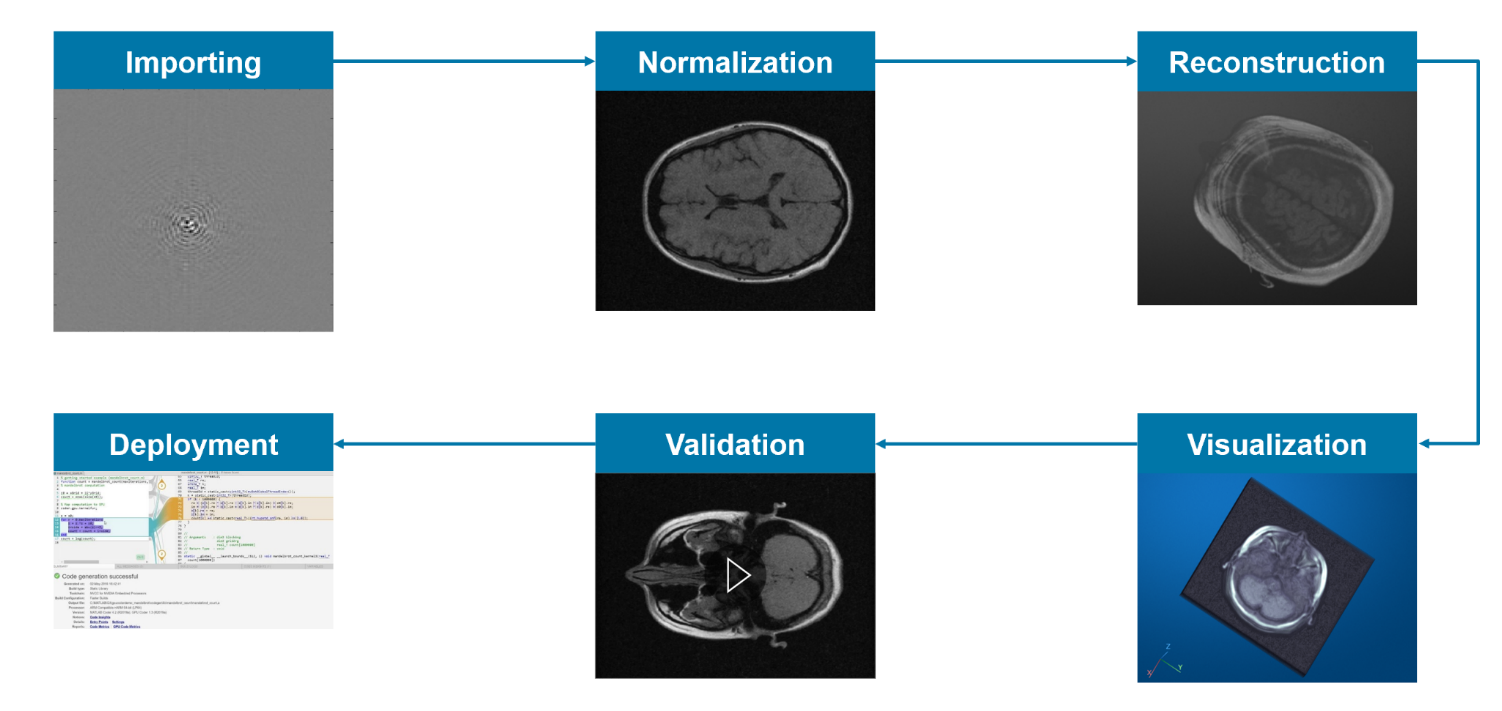
MRI k-space in a nutshell – an MRI scanner uses controlled RF & gradient pulses to fill k-space (frequency data). The inverse 2D FFT then produces the final image. Efficient reconstruction must balance scan time, image quality, and compute cost.
Why Combine Multiple Reconstruction Approaches?
MRI reconstruction involves trade-offs between acquisition speed, image resolution, and artifact suppression. Traditionally, collecting a fully sampled k-space grid and applying an IFFT yields a high-quality image with minimal aliasing. However, fully sampling k-space is time-consuming, which can prolong scan durations for patients and reduce scanner throughput in busy clinical environments. Modern methods speed up scans by undersampling k-space, but a basic IFFT of undersampled data produces artifacts such as aliasing and blurring that can limit diagnostic quality. More advanced computational techniques are therefore needed to reconstruct images from incomplete data.
Instead of betting on a single “silver bullet” algorithm, our MATLAB workflow incorporates multiple reconstruction strategies in one environment. This approach lets you:
- Establish a reliable baseline: The IFFT method provides ground-truth reconstruction on full data. We use it to validate our pipeline and as a quality benchmark.
- Explore accelerated acquisitions: Compressed sensing (CS) allows scanning with fewer k-space samples and reconstructs images by leveraging sparsity – cutting scan time significantly at the cost of computational effort.
- Leverage AI for improvements: Deep learning with a U-Net network architecture can further enhance reconstruction quality or speed by learning from data, reducing residual artifacts and possibly enabling even faster acquisitions without sacrificing image fidelity.
By unifying all three methods in MATLAB, you get the flexibility to switch or combine approaches as needed. For example, you might start from the IFFT baseline and then compare it to a CS reconstruction or use a deep network to refine a physics-based output. And because these solutions share a common environment, it’s straightforward to integrate them with common tasks like visualization, image post-processing, and deployment.
Baseline Reconstruction with Inverse FFT (IFFT)
We begin with the simplest case: fully sampled k-space data. If all required frequency samples have been acquired, reconstructing an image is as direct as performing a 2D inverse Fourier transform. In MATLAB, we can do this with a few lines of code (including coil combination if multiple receiver coils are used):
% Read complex k-space data from HDF5 file
kspaceData = h5read(filePath, datasetPath);

% Move the zero-frequency component from the center to the corners
% (undo the scanner/vendor-specific k-space centering)
kspaceShifted = ifftshift(ifftshift(kspaceData, 1), 2);

% Construct a complex-valued k-space matrix from real and imaginary parts
kspace = complex(kspaceShifted.r, kspaceShifted.i);

% Perform 2-D inverse Fourier transform to reconstruct coil images
imageC = ifft2(double(kspace));

% Shift reconstructed images so that the image center appears in the middle
imageC = fftshift(fftshift(imageC, 1), 2);

% Combine multiple receiver coils using Root-Sum-of-Squares (RSS)
% Coil dimension is assumed to be the 3rd dimension
reconImage = sqrt(sum(abs(imageC).^2, 3));

% Remove singleton dimensions to obtain the final image matrix
reconImage = squeeze(reconImage);
imshow(abs(gather(reconImage)), []);              % display magnitude image
This baseline IFFT reconstruction is fast, deterministic, and rooted in the physics of MRI. With fully sampled data, it produces a high-quality image that can serve as our reference. However, the need to capture all of k-space means long scan times in practice. Next, we look at how to get good images faster by collecting less data and using smarter reconstruction algorithms.
Compressed Sensing: Faster Scans with Sparse Reconstruction
Compressed Sensing (CS) is a technique that enables accurate reconstructions from significantly fewer samples by exploiting sparsity in some transform domain. For MRI, a common approach is to assume the image has a sparse representation in the wavelet domain. By undersampling k-space (skipping many phase-encode lines), we speed up acquisition; then, an iterative algorithm recovers the image by enforcing wavelet sparsity and consistency with the measured data.
In our workflow’s CS example, we simulate an undersampled acquisition (e.g., retaining 25% of the original k-space points in a variable-density random pattern). The reconstruction uses an iterative refine-and-threshold algorithm:
% Initialize storage for compressed sensing reconstructions
im_cs = zeros(size(kspace_data));

% Reconstruct each coil and frame independently
for frame = 1:num_frames
    for coil = 1:num_coils

        % Apply undersampling mask in k-space
        undersampled_data = kspace_data(:,:,coil,frame) .* mask_vardens;

        % Initial image reconstruction from undersampled data
        im_cs(:,:,coil,frame) = ifft2s(undersampled_data);

        % Apply coil sensitivity map
        im_cs(:,:,coil,frame) = ...
            im_cs(:,:,coil,frame) .* coilSensitivityMaps(:,:,coil,frame);

        % POCS-based compressed sensing reconstruction
        for iter = 1:num_iters

            % Transform to wavelet domain and enforce sparsity
            [C, S] = wavedec2(im_cs(:,:,coil,frame), 2, 'db1');
            C_thresh = wthresh(C, 's', threshold);
            im_cs(:,:,coil,frame) = waverec2(C_thresh, S, 'db1');

            % Enforce k-space data consistency
            kspace_estimate = fft2s(im_cs(:,:,coil,frame));
            kspace_estimate(mask_vardens) = ...
                undersampled_data(mask_vardens);

            % Update image estimate
            im_cs(:,:,coil,frame) = ifft2s(kspace_estimate);
        end
    end
end

% Combine all coils using Root-Sum-of-Squares (RSS)
rss_CSimage = sqrt(sum(abs(im_cs).^2, 3));

% Remove singleton dimensions
rss_CSimage = squeeze(rss_CSimage);
How it works: The loop alternates between enforcing measured data (swapping in the acquired k-space lines each iteration) and enforcing image sparsity (zeroing out small wavelet coefficients). Over iterations, the image converges as missing information is filled in by the constraints. The result is a high-quality image reconstructed from a fraction of the data.
If we directly applied an IFFT to undersampled data, we would see strong artifacts due to violation of the Nyquist sampling criterion. With compressed sensing, many of those artifacts are suppressed and the image quality can approach the fully sampled baseline, even when only a fraction of the original k-space samples are acquired. Depending on the sampling pattern, pulse sequence, scanner constraints, and reconstruction setup, this can support meaningful scan-time reductions while helping preserve image quality.
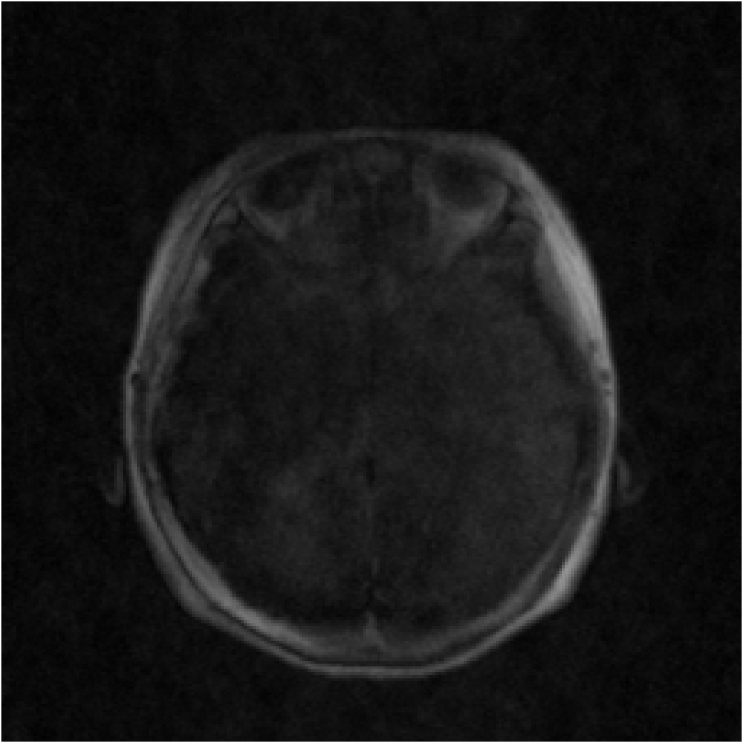
Compressed sensing reconstruction of a representative T1-weighted MRI slice from undersampled, low-SNR input k-space data. The image shows how sparsity-based reconstruction can suppress undersampling artifacts while preserving major anatomical structures.
Note: The above code uses functions from Wavelet Toolbox™ (wavedec2, waverec2) and can automatically leverage the Parallel Computing Toolbox™ to run on a GPU if available (via gpuArray). The iterative CS algorithm is more computationally heavy than IFFT, but GPU acceleration can make it practical for routine use.
Deep Learning Reconstruction with U-Net
Our third approach uses deep learning to push MRI reconstruction further. Instead of relying on hand-crafted transforms or optimization, we train a U-Net (a type of convolutional neural network) to learn the transformation from incomplete data to fully reconstructed image. U-Nets are well-suited for image-to-image tasks like segmentation and, here, reconstruction, thanks to their encoder-decoder structure with skip connections that captures both global context and fine details.
In our MATLAB example, we feed the network zero-filled IFFT reconstructions of undersampled data as inputs and the corresponding fully sampled images as targets. Using the Deep Learning Toolbox™, we can set up and train the U-Net as follows:
% Define a custom U-Net architecture for MRI reconstruction
lgraph = createCustomUNet([256 256 18], 18);

% Specify training parameters
options = trainingOptions("adam", ...
    InitialLearnRate = 1e-3, ...
    MaxEpochs = 600, ...
    MiniBatchSize = 12);

% Train the network using undersampled and reference images
net = trainNetwork(inputDataTrain, groundTruthDataTrain, ...
                   lgraph, options);

% Reconstruct images using the trained network
reconDL = predict(net, inputDataTest);
What’s happening? We define a custom U-Net architecture for image-to-image regression and train it on paired data: zero-filled reconstructions from undersampled k-space as inputs and fully sampled reconstructions as targets. The encoder-decoder structure with skip connections helps the network capture both global context and fine image details. Training options such as the optimizer, learning rate, number of epochs, and mini-batch size control the learning process. When a supported GPU is available and the execution environment is set appropriately, MATLAB can use GPU acceleration through Parallel Computing Toolbox™. After training, the predict function generates rapid reconstructions for new undersampled inputs.
This deep learning approach learns to map artifact-corrupted, zero-filled reconstructions to reference-quality images. If trained and validated well, the U-Net can reduce residual artifacts compared with conventional undersampled reconstruction and may support higher acceleration factors for a given image-quality target. It also runs very fast at inference because reconstruction is essentially one forward pass through the network. However, deep learning models require representative training data, careful validation, and quality-control checks to ensure that they generalize to new scans and do not introduce unintended artifacts. In practice, combining AI with physics-based methods, such as using a CS reconstruction as an input to the U-Net, can further improve robustness.
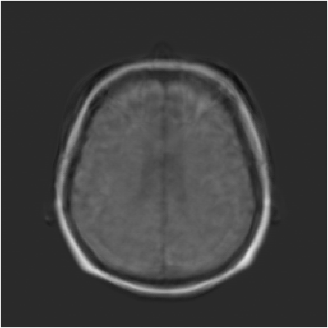
Deep learning reconstruction of a similar representative T1-weighted MRI slice from the same low-SNR input k-space dataset. The U-Net output is generated from an undersampled input reconstruction and is intended to reduce residual artifacts while preserving fine image detail.
Verification, Validation, and Deployment
Developing these algorithms is only part of the story – practical MRI workflows also require rich visualization and an eye towards deployment:
- Automatic Testing and Verification: Because our three methods are implemented in one environment, we can easily create test scripts to verify that each reconstruction matches expected results (within tolerance) or to measure performance (like PSNR, SSIM) across a dataset. This can be integrated into a CI/CD pipeline (Continuous Integration/Deployment) to ensure code changes don’t break the pipeline.
- Interactive Visualization and Validation: MATLAB’s Medical Imaging Toolbox™ provides apps and functions to explore 2D slices and 3D volumes, adjust colormaps (colormap), and even use cinematic volume rendering (volshow). This helps in visually validating results side by side: for example, comparing a CS reconstruction to the IFFT baseline, or overlaying error maps to spot differences.
- GPU Code Generation and Deployment: A standout feature is the ability to automatically generate C/C++ and CUDA® code from our MATLAB algorithms for deployment with IEC 62304 certification support. Using MATLAB Coder™ and GPU Coder™, we can translate the IFFT, CS, or U-Net reconstruction into highly optimized code for embedded applications or integration into an MRI scanner’s software. For instance, we can generate a MEX function or a standalone library from our MATLAB code with just a few commands. The image below shows a snippet of the code generation process in MATLAB:
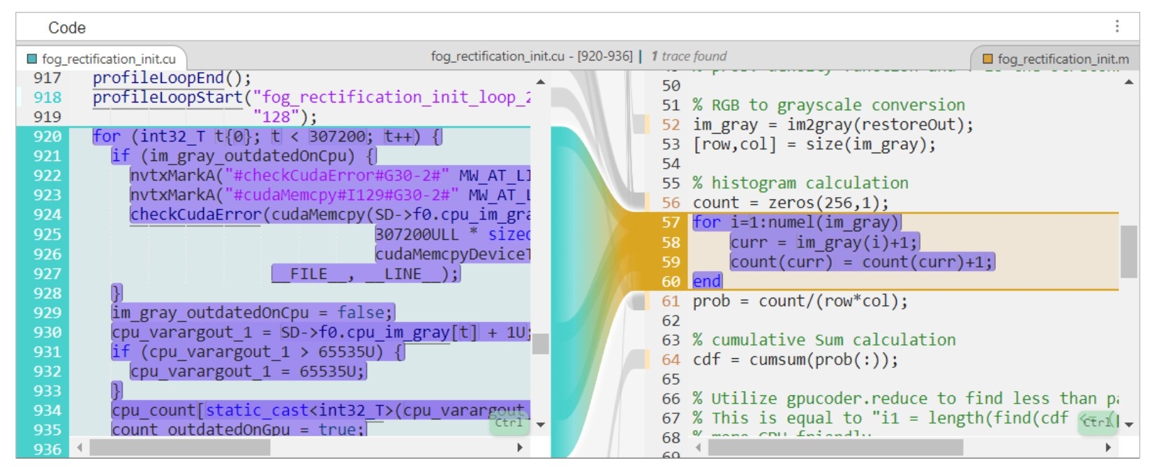
GPU code generation in MATLAB for the IFFT reconstruction algorithm. The code generator converts our MATLAB reconstruction function into a C/CUDA implementation (left: generated code preview and analysis) and reports a successful build (bottom). This enables integrating the proven algorithm into production systems, such as scanner software, with minimal manual coding.
Thanks to GPU acceleration and code generation, MRI reconstruction methods developed in MATLAB can scale from desktop prototyping to execution on specialized hardware. For example, once a U-Net is trained and validated in MATLAB, GPU Coder can help deploy inference code that uses optimized NVIDIA® libraries such as cuDNN and TensorRT, reducing the need to hand-code the inference engine.
Conclusion and Key Takeaways
By combining classical and AI-based reconstruction techniques in a single MATLAB workflow, we can address the diverse needs of modern MRI systems. A unified environment streamlines the process: raw data import, reconstruction, testing, verification, visualization, validation, and certification can all be done in one place, and when it’s time to deploy, the same code is ready for automatic translation to C/CUDA.
In summary, this workflow shows how MATLAB can support MRI reconstruction from early experimentation to deployment:
- IFFT reconstruction provides a fast and reliable baseline for fully sampled data.
- Compressed sensing enables accelerated acquisitions by combining undersampling, sparsity, and data-consistency constraints.
- Deep learning can help reduce artifacts in undersampled reconstructions when trained and validated with representative data.
- GPU acceleration and code generation help bridge the gap between research prototypes and deployable reconstruction pipelines.
We hope this example has shown how classic reconstruction techniques and AI can reinforce each other. By exploring baseline, compressed sensing, and deep learning methods within a unified setting, engineers are empowered to iterate quickly and tailor MRI reconstruction workflows to achieve both faster scans and high image quality, all while maintaining a clear path to real-world deployment.
Try the examples yourself: MRI Reconstruction in MATLAB
- 범주:
- Deep Learning



댓글
댓글을 남기려면 링크 를 클릭하여 MathWorks 계정에 로그인하거나 계정을 새로 만드십시오.