Pinecode: Creating pinecones with Fibonacci spirals
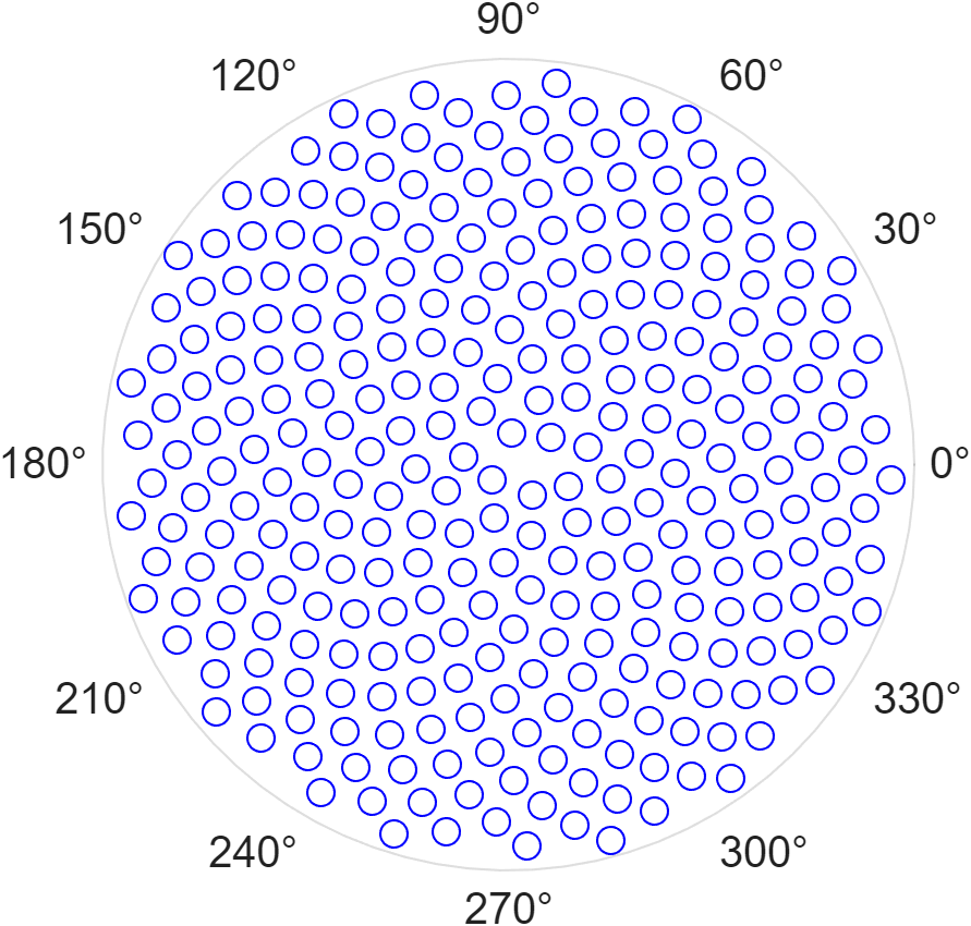
Today we explore phyllotactic spirals, a naturally emerging pattern found in densely packed plant structures such as pineapples, sunflowers, and pinecones. This generative spiral is based on tau, a constant angular offset between successive seeds or scales. When tau equals 2π times the golden ratio, $\frac{1+\sqrt{5}}{2}\approx 1\ldotp 618$ the pattern is known as a Fibonacci spiral. Experiment with different values of tau to see how the spirals transform.

tau = pi*(1+sqrt(5));
n = 1:300;
r = sqrt(n);
theta = n * tau;
polarscatter(theta,r,'bo')
Eric applies this principle to the 3D Cartesian domain in his parameterized pinecode.
 |
Guest Writer: Eric Ludlam Eric, a seasoned MATLAB graphics expert, shares his approach to replicating the natural patterns of a pinecone through code. Learn about pinecone geometry and the efficacy of parameterized graphics. See Eric's full bio on our contributors page. |
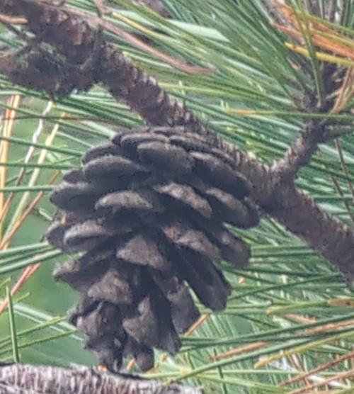
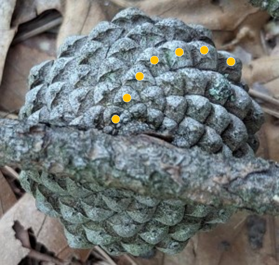
Let's explore a graphics algorithm for creating a pinecone. Here are a couple pictures of pinecones I found. This first was on the coast in Maine, and the second I found along a hiking trail near the MathWorks campus in Natick, Massachusetts.


Pinecones are made of "scales", which you can think of as petals on a flower. In this article, "scale" specifically refers to these structures on the pinecone and not to the common mathematical transformation.
The pinecone pictured on the left has a shape like an upside-down teardrop. The scales are wide and get smaller and more densely packed near the base. The base of the pinecone on the right shows how the scales radiate outward in a Fibonacci spiral, highlighted with yellow dots.
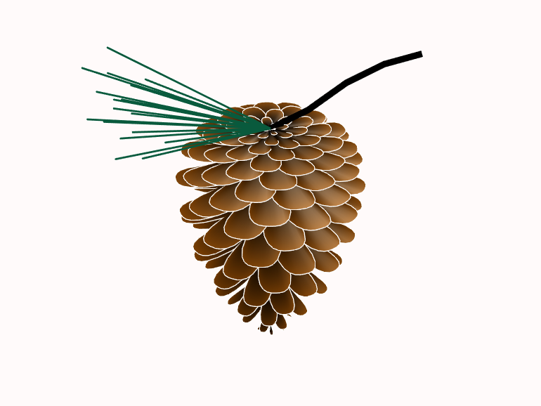
The pinecone algorithm below attempts to replicate these patterns in a single surface object. It starts with a Fibonacci spiral which helps us compute the locations of the tips for each of the scales. Next, we compute the shape of one scale and replicate that shape for each location computed in our spiral.
At the end, I add a little branch and some pine needles using a line and patch.
If you open this blog post in MATLAB Online using the link below, all the parameters at the beginning of the script can be manipulated with sliders and color pickers making it easy for you to design your own pinecone!
Click here to try it!
% Pinecone Attributes
nscales = 140; % Number of scales
height = 2.5; % Height of inner part of pinecone
swt = 0.3; % Scale width in theta
sth = 0.2; % Scale thickness (as a curve in height)
stilt = 1.2; % From inside to outside, tile of each scale
nn = 18; % Number of needles
% Exponents for curves
hexp = 2.8; % scale density over height
rexp = 2; % radius shape across height
scexp = 3; % scale rounded shape (end)
suexp = 3; % scale roundness in height
stexp = 2.1; % scale tilt for height
stuexp = 2; % scale thickness of U by height
cexp = 2; % color gradient
% Colors
brown1 = [0 0 0]; % Dark center color
brown2 = [0.470 0.240 0.010]; % Brigher outer color
edge = [1 1 1]; % Scale edging
green = [0.060 0.590 0.400]; % Pine Needles
% Resolution
vps = 17; % verts per scale : An odd number so 1 vert is in center
vpr = 20; % verts per radius
% Scale locations
FIB = (1+sqrt(5))*(1:nscales); % Fibonacci golden ratio sequence as factor of pi
H = linspace(0,1,nscales).^hexp*height; % Height of the root of each scale
R = 1-abs(linspace(-1,1,nscales).^rexp); % Radius of pinecone over height
U = 1-abs(linspace(-1,1,nscales).^stuexp); % Thickness of scale U shape by height
% Geometry of the scales at the locations
ST = reshape((linspace(-.5,.5,vps)*swt+FIB')', 1,[]); % Scale Theta
SR = reshape(((1-abs(linspace(-1,1,vps).^scexp)).*R')',1,[]); % Scale Radii
SH = reshape((ones(1,vps).*H'+abs(linspace(-1,1,vps).^suexp.*U')*sth)',1,[]); % Scale Height
MR = linspace(0,1,vpr)'.*SR;
% Compute final geometry of the pinecone.
X = cospi(ST).*MR;
Y = sinpi(ST).*MR;
Z = SH.*ones(vpr,1)+MR.*linspace(0,1,vps*nscales).^stexp*stilt;
C = linspace(0,1,vpr).^cexp'.*ones(1,vps*nscales);
% Plot pinecone
set(gcf,'Color','#fffafa'); % Snow
plot3(X(end,:),Y(end,:),-Z(end,:),'-','Color',edge);
surface(X,Y,-Z,C,'EdgeColor','none');
shading interp
% Dark center to Brown colormap
colormap(interp1([1 256],[brown1; brown2],1:256));
% Branch
bx = [ 0 .5 1 1.5 2 ];
by = [ 0 0 0 0 0 ];
bz = [ 0 .05 .2 .25 .2 ];
line('XData',bx,'YData',by,'ZData',bz,'Color',brown1, 'LineWidth',5);
% Pine Needles
NT = linspace(0,5,nn)';
NR = linspace(.1,.8,nn)';
NV = [ 0 0 0
-ones(nn,1)*2, cospi(NT).*NR, sinpi(NT).*NR+.9 ];
NF = [ ones(nn,1) (1:nn)'+1 ];
patch('Vertices',NV,'Faces',NF,'EdgeColor',green,'FaceColor','none',...
'LineWidth',1.5);
% Setup Axes
set(gca,'Position',[0 0 1 1],'Clipping','off');
daspect([1 1 1]);
axis([-1.3 1.3 -1.3 1.3 -height+.2 .5],'off')
material([.6 1 .3])
lighting gouraud
light('Position',[13.2 7.2 16.5]);


댓글
댓글을 남기려면 링크 를 클릭하여 MathWorks 계정에 로그인하거나 계정을 새로 만드십시오.