
How the Tiger got its Stripes
How the Tiger got its Stripes
A couple of years ago, I visited Bletchley Park. There are lots of interesting things to see there, like old Enigma machines and a working replica of the bombe. But I was also impressed by the collection of papers which Alan Turing wrote. It amazed me that he could find time to write papers on subjects like computing the  function with all of the other work he was doing during the war.
But I think that my favorite Turing paper is one he wrote after the war called The Chemical Basis of Morphogenesis. It describes an idea he had for how all of the different patterns on the skins of various animals are formed. It's really a very simple idea. You have two chemicals which are distributed nonuniformly through the skin of the animal. They react with each other, and they each diffuse from areas with high concentrations to areas with low concentrations. It turns out that fiddling the reaction rates and the diffusion rates can yield all sorts of different patterns which look very similar to patterns you see in nature.
This system came to be known as a two-component reaction diffusion system. There are a couple of different versions of this now, but one of the most interesting is the Gray-Scott model.
Let's try writing a simulation of the Gray-Scott model in MATLAB. We'll start from a wonderful version which Karl Sims wrote for the Connection Machine. The equations are the following:


Where A and B are the concentrations of our two chemicals, and k and f are the "kill" and "feed" rates.
You can write this pretty directly in MATLAB like this:
Anew = Aold + (da*del2(Aold) - Aold.*Bold.^2 + f*(1-Aold))*dt;
Bnew = Bold + (db*del2(Bold) + Aold.*Bold.^2 - (k+f)*Bold)*dt;
Where Aold and Bold are the concentrations of the two chemicals at the previous time step and Anew and Bnew are the concentrations at the next time step.
We need to make one tweak though. MATLAB's del2 operator clamps at the edges of the grid. The one which Karl used originally did a "toroidal wrap". This means that cells on the right side were treated as if they were adjacent to cells on the left and cells on the top were treated as if they were adjacent to cells on the bottom. There are a couple of ways to implement this in MATLAB. I'm going to do it using circshift with the following function:
function out = my_laplacian(in)
  out = -in ...
      + .20*(circshift(in,[ 1, 0]) + circshift(in,[-1, 0])  ...
      +      circshift(in,[ 0, 1]) + circshift(in,[ 0,-1])) ...
      + .05*(circshift(in,[ 1, 1]) + circshift(in,[-1, 1])  ...
      +      circshift(in,[-1,-1]) + circshift(in,[ 1,-1]));
We'll use these feed and kill rates
f=.055;
k=.062;
And we'll need a couple of other variables.
% Diffusion rates
da = 1;
db = .5;
% Size of grid
width = 128;
% 5,000 simulation seconds with 4 steps per simulated second
dt = .25;
stoptime = 5000;
We'll use the following function to set the initial conditions, but you can use any other pattern of values in the range [0 1] which isn't too uniform.
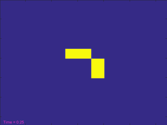
function [t, A, B] = initial_conditions(n)
  t = 0;
  % Initialize A to one
  A = ones(n);
  % Initialize B to zero which a clump of ones
  B = zeros(n);
  B(51:60 ,51:70) = 1;
  B(61:80,71:80) = 1;
OK, let's run the simulation.
[t, A, B] = initial_conditions(width);

tic
nframes = 1;
while t<stoptime
    anew = A + (da*my_laplacian(A) - A.*B.^2 + f*(1-A))*dt;
    bnew = B + (db*my_laplacian(B) + A.*B.^2 - (k+f)*B)*dt;
    A = anew;
    B = bnew;
    t = t+dt;
    nframes = nframes+1;
end
And we'll draw the results as an image
axes('Position',[0 0 1 1])
axis off

% Add a scaled-color image
hi = image(B);
hi.CDataMapping = 'scaled';

delta = toc;
disp([num2str(nframes) ' frames in ' num2str(delta) ' seconds']);
20001 frames in 16.9648 seconds
That took about 17 seconds. But we only got to see the final picture. It'd be a lot cooler if we could see the simulation as it was running.
To do that, we'll create the image at the beginning and set its CData in the inner loop.
[t, A, B] = initial_conditions(width);

% And a text object to show the current time.
ht = text(3,width-3,'Time = 0');
ht.Color = [.95 .2 .8];
drawnow

tic
nframes = 1;
while t<stoptime
    anew = A + (da*my_laplacian(A) - A.*B.^2 + f*(1-A))*dt;
    bnew = B + (db*my_laplacian(B) + A.*B.^2 - (k+f)*B)*dt;
    A = anew;
    B = bnew;
    hi.CData = B;
    t = t+dt;
    ht.String = ['Time = ' num2str(t)];
    drawnow
    nframes = nframes+1;
end
delta = toc;
disp([num2str(nframes) ' frames in ' num2str(delta) ' seconds']);
20001 frames in 118.4511 seconds
That looked pretty cool, but it took more than 100 seconds. That seems like a lot! Can't we make the simulation run reasonably fast and still get to see it?
When we ran the simulation without the graphics, we were able to do more than 1,000 simulation time steps per second. But the graphics card on my system can't display frames that quickly. It needs to do a bunch of work to move the data from MATLAB's memory system to the memory system of the graphics card. In this example, it can only do that at about 200 frames per second.
But in a way, that's OK. Our eyes can't really see things changing at much more than 30 frames per second, and most computer monitors don't refresh a lot faster than that. So what if we didn't send ALL of the simulation time steps to the graphics card?
Traditionally we've done this in MATLAB by keeping track of the current time and using that to decide whether we need to call drawnow. Here's how it looks for trying to hit a framerate of 24 frames per second.
[t, A, B] = initial_conditions(width);

targetframerate = 24;
frametime = 1/(24*60*60*targetframerate);
nextframe = now + frametime;
tic
nframes = 1;
while t<stoptime
    anew = A + (da*my_laplacian(A) - A.*B.^2 + f*(1-A))*dt;
    bnew = B + (db*my_laplacian(B) + A.*B.^2 - (k+f)*B)*dt;
    A = anew;
    B = bnew;
    hi.CData = B;
    t = t+dt;
    ht.String = ['Time = ' num2str(t)];
    if now > nextframe
        drawnow
        nextframe = now + frametime;
    end
    nframes = nframes+1;
end
delta = toc;
disp([num2str(nframes) ' frames in ' num2str(delta) ' seconds']);
20001 frames in 27.1881 seconds
That took less than 25 seconds, which is a lot closer to our original simulation. But that code has gotten kind of ugly, hasn't it? It be nice if this was simpler.
In R2015a there's a new drawnow option which does this for you! It's called "limitrate", and you use it like this:
[t, A, B] = initial_conditions(width);

tic
nframes = 1;
while t<stoptime
    anew = A + (da*my_laplacian(A) - A.*B.^2 + f*(1-A))*dt;
    bnew = B + (db*my_laplacian(B) + A.*B.^2 - (k+f)*B)*dt;
    A = anew;
    B = bnew;
    hi.CData = B;
    t = t+dt;
    ht.String = ['Time = ' num2str(t)];
    drawnow limitrate
    nframes = nframes+1;
end
delta = toc;
disp([num2str(nframes) ' frames in ' num2str(delta) ' seconds']);
20001 frames in 23.8246 seconds
That's about as simple as our first try, and it runs in just 20 seconds, which is getting pretty close to the original version with no graphics, but the animation still looks good on screen.
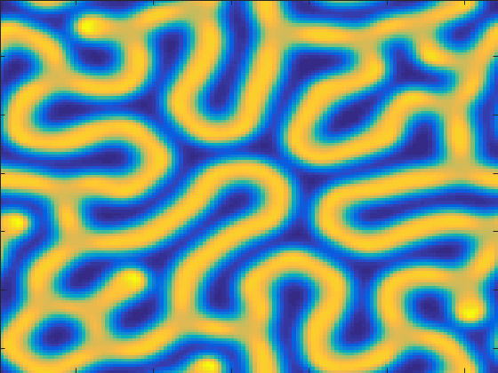
Now that we've built a simulator for the Gray-Scott equations, try using different values for the kill and feed rates. See if you can create patterns that look like real animal coats.
Here are some of my favorites:
f = .018
k = .051
.gif)
f = 0.026
k = 0.053
.gif)
f = 0.055
k = 0.063
.gif)
- カテゴリ:
- Animation

