What is a Contour?
What is a Contour?
Last year we explored how surfaces perform interpolation. Today we're going to take a look at some closely related functions; the contour family. The family of contour functions consists contour, contour3, and contourf and a couple of other minor ones.
We'll start with a simple 7x5 array. We'll create a surface and a filled contour using contourf.
rng default
z = randn(7,5)

a1 = subplot(1,2,1);
h = surf(z);
h.FaceColor = 'interp';
axis tight

a2 = subplot(1,2,2);
contourf(z)
z =

    0.5377    0.3426    0.7147   -1.2075    0.2939
    1.8339    3.5784   -0.2050    0.7172   -0.7873
   -2.2588    2.7694   -0.1241    1.6302    0.8884
    0.8622   -1.3499    1.4897    0.4889   -1.1471
    0.3188    3.0349    1.4090    1.0347   -1.0689
   -1.3077    0.7254    1.4172    0.7269   -0.8095
   -0.4336   -0.0631    0.6715   -0.3034   -2.9443
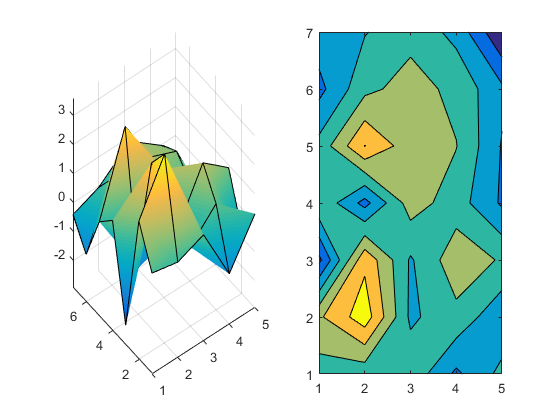
It's hard to see the relationship at first. But if we look straight down on the surface and square up the aspect ratio of the axes (and squint a little) we can see that they are related.
axes(a1)
view(2)
axis([a1 a2],'equal')
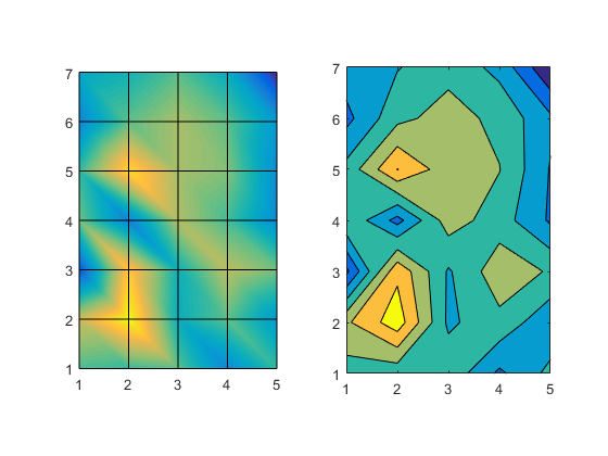
But, they certainly don't look the same though, do they?
It's easier to see what's going on if we look at a single contour level. That's easy to do with contour by setting the LevelList property. With surface we can simulate it by adding a white plane a Z==0 to hide the part of the surface which is below that.
axes(a1)
p = surface([1 5;1 5],[1 1; 7 7],zeros(2));
p.FaceColor = 'white';
p.EdgeColor = 'none';

axes(a2)
contourf(z,'LevelList',0)
axis equal
grid on
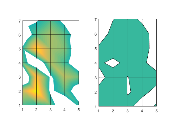
They still don't look like they're showing the same thing though, do they? But look closely. Look at where the curve intersects the grid lines. The intersection points are the same in the two pictures. The differences are all between those intersection points. What we're seeing is the same thing we saw when we looked at surfaces. The interpolation function matters, and surface and contour use different interpolation functions.
Last time we learned about the piecewise linear interpolation that surface uses, and we wrote an interpsurf function to give use more control by using the interp2 function. Let's try using that with interp2's linear method and see if that matches what contour is doing.
axes(a1)
interpsurf(z,'linear')
p = surface([1 5;1 5],[1 1; 7 7],zeros(2));
p.FaceColor = 'white';
p.EdgeColor = 'none';
view(2)
axis tight
axis equal
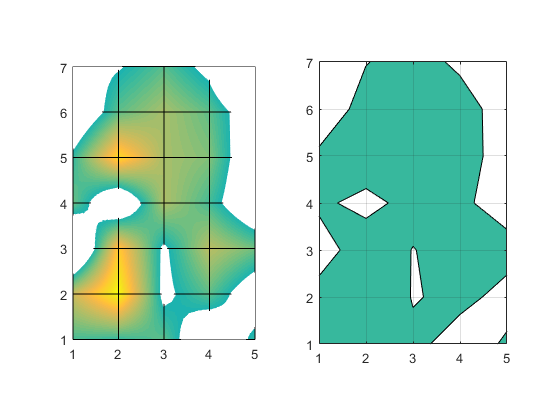
No, they're still not the same. We can see that interpsurf is drawing curves in between the grid lines. You may remember that when we discussed the bilinear interpolation that interp2 is using here, we saw that it's giving us a quadratic equation of this form.
$$f(x,y) = c_1 + c_2 x + c_3 y + c_4 x y$$
This tells us that the curves we're seeing between the grids are actually segments of hyperbolas. But contour is drawing straight lines in between the grid. Its interpolation scheme is basically to do linear interpolation on each of the edges and then draw a straight line connecting them.
But there's another important difference, isn't there? You can see that in the squares where the curve intersects all four sides, there are a couple of different ways to connect the intersections. These are called the ambiguous cases. There are a couple of different ways to decide which way to go in these cases, and the surface and contour functionss don't use the same technique. Can you spot the square where the two algorithms connected the intersections differently?
We can use the same technique we used in the intersurf function to perform our own interpolation on the input to contour like this:
axes(a2)
[x, y] = meshgrid(1:5,1:7);
[x2,y2] = meshgrid(1:.1:5,1:.1:7);
z2 = interp2(x,y,z, x2,y2, 'linear');
contourf(x2,y2,z2,'LevelList',0)
axis equal
grid on
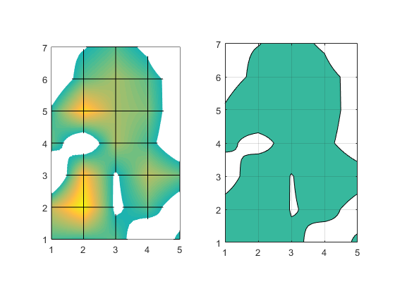
That looks pretty good, and it matches our surface, but when we go back to the default LevelList we can see that it still doesn't look very smooth. That's because bilinear interpolation is only C0 continuous between 2x2 sections. This shows up as sudden changes of direction as the curves cross these boundaries.
axes(a1)
interpsurf(z,'linear')
view(2)
axis tight
axis equal
axes(a2)
contourf(x2,y2,z2)
axis equal
grid on
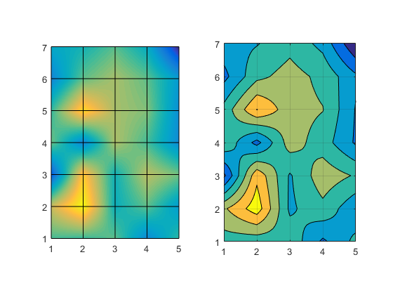
We don't usually notice this too much with surfaces because the colors or lighting tends to soften these discontinuities in the derivative. But the hard edges in a contour make it very noticeable.
What if we switch to a smoother interpolation method? For example, cubic.
axes(a1)
interpsurf(z,'cubic')
view(2)
axis tight
axis equal
axes(a2)
z2 = interp2(x,y,z, x2,y2, 'cubic');
contourf(x2,y2,z2)
axis equal
grid on
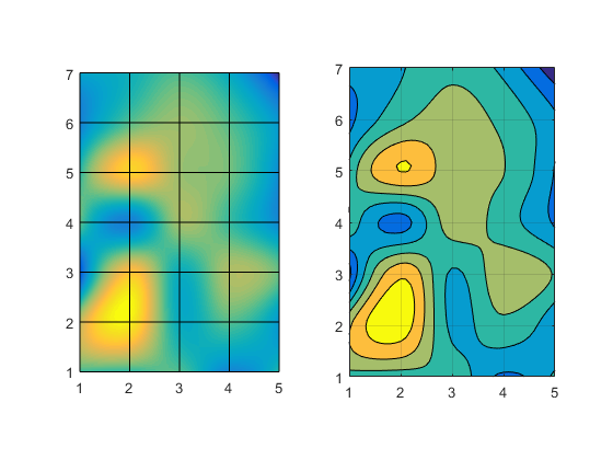
That looks pretty nice, doesn't it? Can you use that to create an interpcontourf function, just like the interpsurf function we created last time? But remember, there is no single "correct" interpolation scheme. You need to know something about the characteristics of your data to know which scheme is most appropriate. In some cases a very smooth interpolation method like cubic can result in a contour which makes your data look smoother than it really should.
The contour and surface functions use the simplest and fastest interpolation schemes for their jobs. That's because you can always do preprocessing up front to get characteristics like smoother interpolation, but you really can't do preprocessing to get performance.
- 类别:
- Geometry


