Locating the US continental divide, part 4 – Ocean masks

作者 Steve Eddins, May 15, 2009

2 次查看（过去 30 天） | 0 个赞 | 0 个评论

Welcome to part 4 of my series on computing the US continental divide. Previously we looked at data import and display, the watershed transform and label matrices, and different kinds of minima.

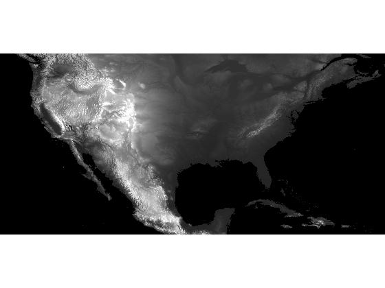
Today we're going to use some binary image manipulation to create an "ocean mask." Let's start by taking a fresh look at some of the pixel values in the DEM (digital elevation model) we've been working with.

s = load('continental_divide');
dem = s.dem_cropped;
display_range = [-500 3000];
imshow(dem, display_range, 'InitialMagnification', 'fit')

What are the pixel values associated with the ocean? You might expect them to be 0. After all, the ocean is at sea level! But a few values at the upper-left corner of the DEM are not 0:

dem(1:5, 1:5)

ans =

   -500   -500   -500   -500   -500
   -500   -500   -500   -500   -500
   -500   -500   -500   -500   -500
   -500   -500   -500   -500   -500
   -500   -500   -500   -500   -500

Are the ocean pixels equal to -500 all the way up to the coast? When I want to inspect pixel values closely, I often use the Pixel Region Tool. Here's a screen shot of the tool showing pixel values along the coast of California:

So the value -500 seems to be used as an ocean marker value. But I prefer not to guess. After some browsing of the online report about this data set, I found this sentence in Section 11: "Every tile contains values of -500 for oceans, with no values between -500 and the minimum value for land noted here."

We can use a simple relational operator to form an ocean mask image.

ocean_mask = dem == -500;
imshow(ocean_mask, 'InitialMagnification', 'fit')

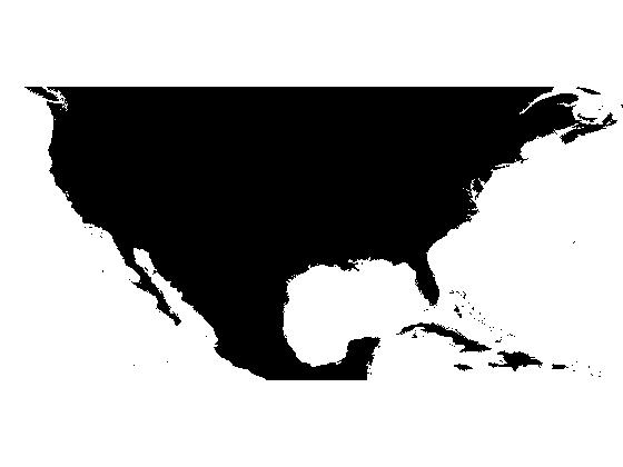
I expected ocean_mask to have just two connected components, corresponding to the Pacific and Atlantic Oceans. But I was surprised:

ocean_mask_labeled = bwlabel(ocean_mask);
max(ocean_mask_labeled(:))

ans =

   835

Oops. More than 800 labeled regions, not two. Let's zoom in the coast of the Gulf of Mexico to see what's going on.

axis([3700 4300 2500 2800])

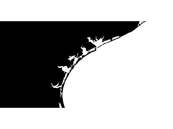
You can see that there are "ocean" pixels that are completely disconnected from the rest of the oceans. How can we identify just the connected components of ocean pixels on the left and right side of the DEM? One method is to use bwselect. This function can find all foreground pixels that are "connected" to a given set of seed pixels. Here I'll use it to find all the "ocean" pixels connected to the upper left and upper right components.

[M, N] = size(dem);
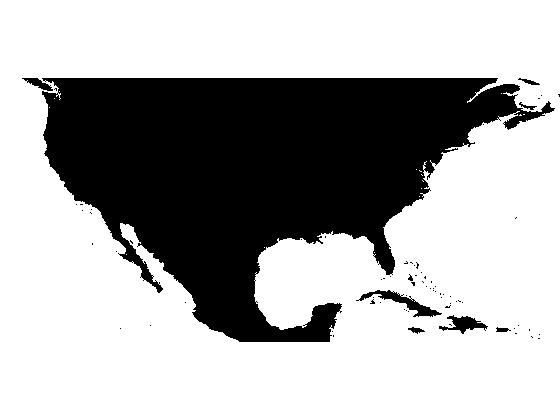
ocean_mask = bwselect(ocean_mask, [1 N], [1 1]);

Here's the same zoomed-in view along the Gulf of Mexico.

imshow(ocean_mask, 'InitialMagnification', 'fit')
axis([3800 4400 2550 2750])

You can see that the interior "ocean pixels" have been removed. Let's add this image to our continental divide MAT-file.

save continental_divide ocean_mask -append

Next time we'll use a technique called minima imposition to modify the DEM so that it contains only two regional minima, one for each ocean.

About this Series

This series explores the problem of computing the location of the continental divide for the United States. The divide separates the Atlantic and Pacific Ocean catchment basins for the North American continent.

As an algorithm development problem, computing the divide lets us explore aspects of data import and visualization, manipulating binary image masks, label matrices, regional minima, and the watershed transform.

Part 1 - Introduction. Data import and display. multibandread, imshow.

Part 2 - Watershed transform. watershed, label2rgb.

Part 3 - Regional minima. imerode, imregionalmin.

Part 4 - Ocean masks. binary image manipulation, bwselect.

Part 5 - Minima imposition. imimposemin.

Part 6 - Computing and visualizing the divide. watershed, label2rgb, bwboundaries.

Part 7 - Putting it all together. One script that does everything, from data import through computation and visualization of the divide.

Data credit: GLOBE Task Team and others (Hastings, David A., Paula K. Dunbar, Gerald M. Elphingstone, Mark Bootz, Hiroshi Murakami, Hiroshi Maruyama, Hiroshi Masaharu, Peter Holland, John Payne, Nevin A. Bryant, Thomas L. Logan, J.-P. Muller, Gunter Schreier, and John S. MacDonald), eds., 1999. The Global Land One-kilometer Base Elevation (GLOBE) Digital Elevation Model, Version 1.0. National Oceanic and Atmospheric Administration, National Geophysical Data Center, 325 Broadway, Boulder, Colorado 80305-3328, U.S.A. Digital data base on the World Wide Web (URL: http://www.ngdc.noaa.gov/mgg/topo/globe.html) and CD-ROMs.

Published with MATLAB® 7.8