Last week I showed a couple of continuous-time Fourier transform pairs (for a cosine and a rectangular pulse). Today I want to follow up by discussing one of the ways in which reality confounds our expectations and causes confusion. Specifically, when we're talking about real signals and systems, we never truly have an infinitely long signal.

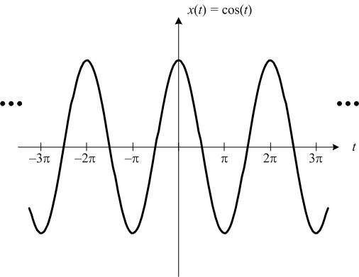
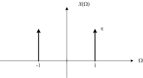
To refresh your memory, here are the ideal cosine signal and its continuous-time Fourier transform plots again:

The dots at the left and right of the cosine plot are meant to remind you that the cosine signal is defined for all t.

But what if we modify the cosine signal so that we have only a finite number of periods? Let's start with a single period, for example.

% N = number of desired cosine periods
N = 1;

t1 = -N*pi;
t2 = N*pi;
t = linspace(t1, t2, 1000);
x = cos(t);
plot(t,x)
ylim([-1.25 1.25])
xlabel('t')
title('x(t) = cos(t)')

In signal processing jargon you'll see this kind of signal referred to as a windowed cosine with a rectangular window. That is, the signal is an infinite-extent cosine multiplied by a finite-extent rectangular pulse.

If I've done my math correctly, the continuous-time Fourier transform of a cosine signal truncated to a finite number of periods is:

where N is the number of periods.

(And if I haven't done my math correctly, I'm sure a sharp-eyed reader will let me know. I feel like I'm back at Georgia Tech working on homework sets. Except that I'm doing it during the day instead of late at night.)

omega = linspace(-5.5, 5.5, 500);
X = sin(pi*N*(omega-1))./(omega-1) + sin(pi*N*(omega+1))./(omega+1);
plot(omega, X)
title('X(\Omega)')
xlabel('\Omega (rad/s)')

Well, that doesn't look very much like the continuous-time Fourier transform for the ideal cosine! If you run this code yourself, try zooming in to look closely at those peaks. You'll see they aren't even located precisely at 1.0 rad/s.

Let's try 10 periods.

N = 10;
t1 = -N*pi;
t2 = N*pi;
t = linspace(t1, t2, 1000);
x = cos(t);
plot(t,x)
ylim([-1.25 1.25])
xlabel('t')
title('x(t) = cos(t)')

omega = linspace(-5.5, 5.5, 500);
X = sin(pi*N*(omega-1))./(omega-1) + sin(pi*N*(omega+1))./(omega+1);
plot(omega, X)
title('X(\Omega)')
xlabel('\Omega (rad/s)')

That's closer, but there's still a lot of funny stuff going on. The more periods we use, the closer the Fourier transform gets to the ideal case, but for any finite number of periods we're going to get this decaying ripple effect.

Later, when we start constructing synthetic spatial sinusoid images (like in this post), and what we see in the frequency domain looks "messy," this is one of the big reasons. All our images have finite extent! We'll be coming back to this idea in future posts.

Have you heard the term bandlimited? It refers to a signal that has no frequency energy above a certain cut-off frequency. Ponder this notion: No finite-extent signal is bandlimited. That is, any signal that is nonzero over only a finite portion of the time domain has nonzero frequency energy across the entire frequency domain.

I think that next time I'll be ready to start talking about the discrete-time Fourier transform, or DTFT. Conceptually we are traveling methodically toward the discrete Fourier transform, or DFT, which is what the MATLAB function fft computes. Along the way we'll figure out how all three forms (continuous-time Fourier transform, discrete-time Fourier transform, and discrete Fourier transform) relate to each other.

Get the MATLAB code

Published with MATLAB® 7.9