
Image-based graphs
Last time I showed you the basics of using the new graph theory functionality in MATLAB R2015b. Today I want to talk about some functions I put on the File Exchange for making graphs from images. Those of you working with graph-based image analysis algorithms might find them useful. I would be very interested in receiving feedback on these functions.
The function imageGraph creates a graph representing the neighbor relationships for every pixel in an image with a specified size. imageGraph3 does the same thing for a 3-D image array.
The function binaryImageGraph creates a graph representing the neighbor relationships for every foreground pixel in a binary image. binaryImageGraph3 creates a graph from a 3-D binary image array.
The function plotImageGraph plots a graph created by imageGraph or binaryImageGraph with the graph nodes arranged on a pixel grid.
Finally, the function adjacentRegionGraph creates a graph from a label matrix defining image regions. The graph represents the region adjacency relationships.
Contents
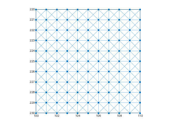
Example: Image graph with 8-connected pixels
Create a graph for a 480-by-640 image with 8-connected pixels.
g = imageGraph([480 640],8)
g =

  graph with properties:

    Edges: [1225442x2 table]
    Nodes: [307200x3 table]
Graph nodes contain the x-coordinate, y-coordinate, and linear index of the corresponding image pixels.
g.Nodes(1:5,:)
ans =

    x    y    PixelIndex
    _    _    __________

    1    1    1
    1    2    2
    1    3    3
    1    4    4
    1    5    5
Plot the image graph using plotImageGraph.
plotImageGraph(g)
axis([100 110 220 230])
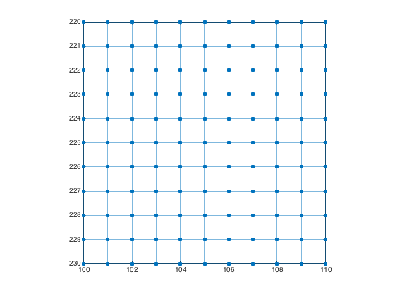
Example: Image graph with 4-connected pixels
Create a graph for a 480-by-640 image with 4-connected pixels.
g = imageGraph([480 640],4)
g =

  graph with properties:

    Edges: [613280x2 table]
    Nodes: [307200x3 table]
plotImageGraph(g)
axis([100 110 220 230])
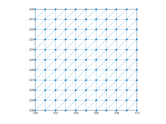
Example: Image graph with special connectivity
Use a 3-by-3 connectivity matrix to create an image graph with 6-connected pixels. Each pixel is connected to its north, northeast, east, south, southwest, and west neighbors.
conn = [0 1 1; 1 1 1; 1 1 0];
g = imageGraph([480 640],conn);
plotImageGraph(g)
axis([100 110 220 230])
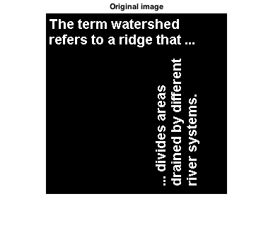
Example: Binary image graph
Create a graph whose nodes are the foreground pixels of the binary image text.png (a sample image that is included with the Image Processing Toolbox).
bw = imread('text.png');
imshow(bw)
title('Original image')
g = binaryImageGraph(bw);
figure
plotImageGraph(g)
axis([60 85 30 45])

Region Graphs
A label matrix defines a set of regions based on each unique element value in the matrix. For example, suppose you had the following label matrix:
L = [10 10 3 4.5 4.5; 10 10 3 4.5 4.5; 20 20 3 15 15; 20 20 3 15 15]
L =

   10.0000   10.0000    3.0000    4.5000    4.5000
   10.0000   10.0000    3.0000    4.5000    4.5000
   20.0000   20.0000    3.0000   15.0000   15.0000
   20.0000   20.0000    3.0000   15.0000   15.0000
This label matrix defines 5 regions:
- A 2-by-2 region in the upper left labeled with the value 10.
- A 2-by-2 region in the lower left labeled with the value 20.
- A one-pixel-wide vertical region in the middle labeled with the value 3.
- A 2-by-2 region in the upper right labeled with the value 4.5.
- A 2-by-2 region at the lower right labeled with the value 15.
The function adjacentRegionsGraph returns a graph with the same number of nodes as labeled regions. Edges in the graph indicate pairs of adjacent regions.
Example: Region graph
Compute an adjacent regions graph. Plot the graph, highlighting the nodes connected to the label 15.
g = adjacentRegionsGraph(L)
g =

  graph with properties:

    Edges: [6x2 table]
    Nodes: [5x1 table]
The graph nodes contain the region labels.
g.Nodes
ans =

    Label
    _____

      3
    4.5
     10
     15
     20
The graph edges contain the labels for each adjacent region pair.
g.Edges
ans =

    EndNodes      Labels
    ________    __________

    1    2        3    4.5
    1    3        3     10
    1    4        3     15
    1    5        3     20
    2    4      4.5     15
    3    5       10     20
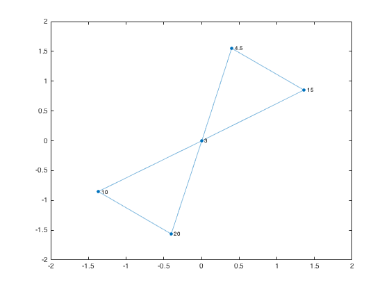
Plot the graph, capturing the GraphPlot object as an output argument.
gp = plot(g,'NodeLabel',g.Nodes.Label)
gp =

  GraphPlot with properties:

     NodeColor: [0 0.4470 0.7410]
    MarkerSize: 4
        Marker: 'o'
     EdgeColor: [0 0.4470 0.7410]
     LineWidth: 0.5000
     LineStyle: '-'
     NodeLabel: {'3'  '4.5'  '10'  '15'  '20'}
     EdgeLabel: {}
         XData: [0.0011 0.4051 -1.3642 1.3629 -0.4048]
         YData: [0.0015 1.5564 -0.8540 0.8538 -1.5577]

  Use GET to show all properties
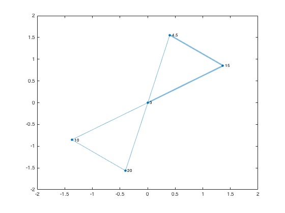
Find the neighbors of the region labeled 15.
node_num = find(g.Nodes.Label == 15);
neighbors_15 = neighbors(g,node_num);
highlight(gp,node_num,neighbors_15)
Next time I plan to show you a graph-based maze solver ... that cheats.
I'd love for you try Image Graphs. Please let me know what you think.
Copyright 2015 The MathWorks, Inc.
Published with MATLAB® R2015b


コメント
コメントを残すには、ここ をクリックして MathWorks アカウントにサインインするか新しい MathWorks アカウントを作成します。