Network Visualization Based on Occlusion Sensitivity
Have you ever wondered what your favorite deep learning network is looking at? For example, if a network classifies this image as "French horn," what part of the image matters most for the classification?
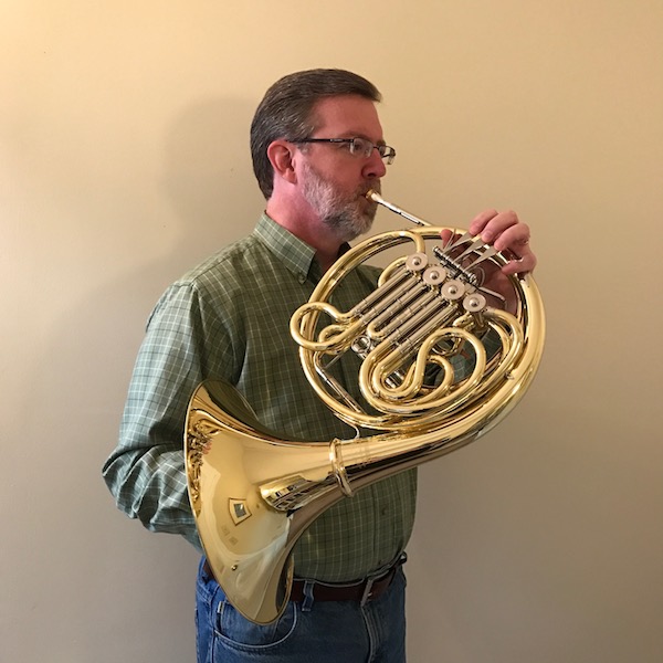
Birju Patel, a developer on the Computer Vision System Toolbox team, helped me with the main idea and code for today's post. Birju has focused on deep learning for the last couple of years. Before that, he worked on feature extraction methods and on optimizing feature matching.
Let's use the pretrained ResNet-50 network for this experiment. (He, Kaiming, Zhang, Xiangyu, Ren, Shaoqing, Sun, Jian. "Deep Residual Learning for Image Recognition." In Proceedings of the IEEE conference on computer vision and pattern recognition, pp. 770-778. 2016.) An easy way to get the ResNet-50 network for MATLAB is to launch the Add-On Explorer (from the HOME tab in MATLAB) and search for resnet.
net = resnet50;
We need to be aware that ResNet-50 expects the input images to be a particular size. The network's initial layer has this information.
sz = net.Layers(1).InputSize(1:2)
sz =

   224   224
The required image size can be passed directly to the imresize function.
url = 'https://blogs.mathworks.com/steve/files/steve-horn.jpg';
rgb = imread(url);
rgb = imresize(rgb,sz);
imshow(rgb)
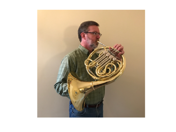
Call classify with the network and the image to see what category the network thinks is most probable.
classify(net,rgb)
ans =

  categorical

     French horn
ResNet-50 thinks I am playing the French horn.
Birju was reading a paper by Zeiler and Fergus about visualization techniques for convolutional neural networks, and in it he came across the idea of occlusion sensitivity. If you block out, or occlude, a portion of the image, how does that affect the probability score of the network? And how does the result vary depending on which portion you occlude?
Let's try it.
rgb2 = rgb;
rgb2((1:71)+77,(1:71)+108,:) = 128;
imshow(rgb2)
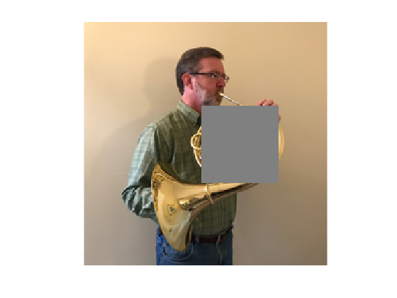
classify(net,rgb2)
ans =

  categorical

     notebook
Hmm. I guess the network "thinks" that gray square looks like a notebook. That region must be important for classifying the image. Now let's try the occlusion in a different spot.
rgb3 = rgb;
rgb3((1:71)+15,(1:71)+80,:) = 128;
imshow(rgb3)
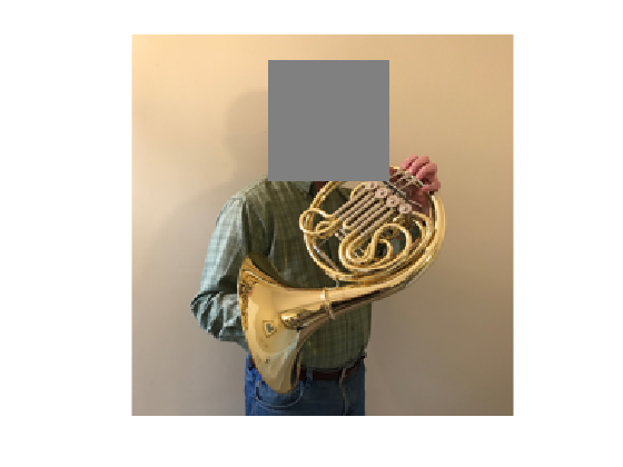
classify(net,rgb3)
ans =

  categorical

     French horn
Hmm. I guess my head is not as important.
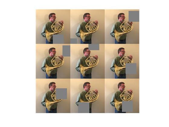
Anyway, Birju wrote some MATLAB code to systematically quantify the relative importance of different images regions to the classification result. His code builds up a large batch of images. For each image in the batch, a different region is occluded. For each location of the occlusion mask, the prediction score of the expected class ("French horn," in this case) is recorded.
Let's make a batch of images with 71x71 regions masked out. Start by computing the corners of all the masks, represented as (X1,Y1) and (X2,Y2).
mask_size = [71 71];
[H,W,~] = size(rgb);

X = 1:W;
Y = 1:H;

[X1, Y1] = meshgrid(X, Y);

X1 = X1(:) - (mask_size(2)-1)/2;
Y1 = Y1(:) - (mask_size(1)-1)/2;

X2 = X1 + mask_size(2) - 1;
Y2 = Y1 + mask_size(1) - 1;
Don't let the mask corners stray outside the image boundaries.
X1 = max(1, X1);
Y1 = max(1, Y1);

X2 = min(W, X2);
Y2 = min(H, Y2);
Make the batch.
batch = repmat(rgb,[1 1 1 size(X1,1)]);

for i = 1:size(X1,1)
   c = X1(i):X2(i);
   r = Y1(i):Y2(i);
   batch(r,c,:,i) = 128; % gray mask.
end
[Note: This batch has more than 50,000 images in it. You'll need a lot of RAM to create and process such a large batch of images all at once.]
Here are a few of the masked images.
montage(batch(:,:,:,randperm(size(X1,1),9)))
Now I'll use predict (instead of classify) to get the prediction scores for each category and for each image in the batch. The 'MiniBatchSize' parameter is used to keep the GPU memory use down. It means that the predict function will send 64 images at a time to the GPU for processing.
s = predict(net, batch, 'MiniBatchSize',64);
size(s)
ans =

       50176        1000
That's a lot of prediction scores! There are 51,529 images in the batch, and there are 1,000 categories. The matrix s has a score for each category and for each image.
We are specifically interested in the prediction scores for the category predicted for the original image. Let's figure out the category index for that.
scores = predict(net,rgb);
[~,horn_idx] = max(scores);
So, here are the French horn scores for every image in the batch:
s_horn = s(:,horn_idx);
Reshape the set of horn scores to be an image and display it.
S_horn = reshape(s_horn,H,W);
imshow(-S_horn,[])
colormap(gca,'parula')
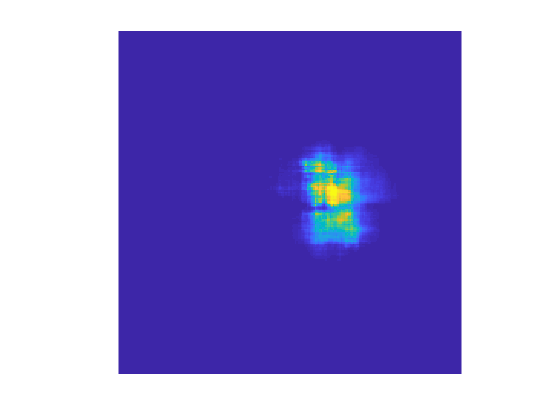
The brightest regions indicate the locations where the occlusion had the biggest effect on the probability score.
Let's find the location that minimizes the "French horn" probability score.
[min_score,min_idx] = min(s_horn);
rgb_min_score = batch(:,:,:,min_idx);
imshow(rgb_min_score)
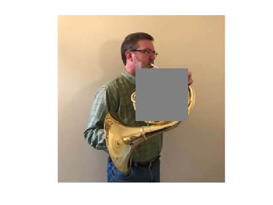
There you go. To recognize a French horn, it's all about the valves and valve slides. It's not about the bell.
A final note on terminology: Some of my horn-playing friends might give me a hard time about calling my instrument a "French horn." According to the International Horn Society, the instrument should just be called "horn." However, the label stored in ResNet-50 is "French horn," and that is the most commonly used term in the United States, where I live.
- Category:
- Deep Learning


Comments
To leave a comment, please click here to sign in to your MathWorks Account or create a new one.