
Deep Learning for Medical Imaging: Malaria Detection
| This post is from Barath Narayanan, University of Dayton Research Institute. Dr. Barath Narayanan graduated with MS and Ph.D. degree in Electrical Engineering from the University of Dayton (UD) in 2013 and 2017 respectively. He currently holds a joint appointment as an Associate Research Scientist at UDRI's Software Systems Group and as an Adjunct Faculty for the ECE department at UD. His research interests include deep learning, machine learning, computer vision, and pattern recognition. |  |
Data Science is currently one of the hot-topics in the field of computer science. Machine Learning (ML) has been on the rise for various applications that include but not limited to autonomous driving, manufacturing industries, medical imaging. Computer Aided Detection (CAD) and diagnosis in medical imaging has been a research area attracting great interest. 3.2 billion people are at risk for contracting malaria across the world (https://www.childfund.org/infographic/malaria/). Detection and diagnosis tools offer a valuable second opinion to the doctors and assist them in the screening process. In this blog, we're applying a Deep Learning (DL) based technique for detecting Malaria on cell images using MATLAB. Plasmodium malaria is a parasitic protozoan that causes malaria in humans and CAD of Plasmodium on cell images would assist the microscopists and enhance their workflow.
Please cite the following article if you're using any part of the code for your research.
Barath Narayanan Narayanan, Redha Ali, and Russell C. Hardie "Performance analysis of machine learning and deep learning architectures for malaria detection on cell images", Proc. SPIE 11139, Applications of Machine Learning, 111390W (6 September 2019); https://doi.org/10.1117/12.2524681
Malaria dataset is made publicly available by the National Institutes of Health (NIH). This dataset contains 27,558 images belonging to two classes (13,779 belonging to parasitized and 13,799 belonging to uninfected). All these images are manually annotated by an expert slide reader at the Mahidol-Oxford Tropical Medicine Research Unit. After downloading the ZIP files from the website and extracting them to a folder called "cell_images", we have one sub-folder per class in "cell_images". Parasitized indicates the presence of plasmodium which is a type of parasitic protozoan indicating the presence of malaria. Since we have equal distribution of both classes, there is no class imbalance issue here.
Load the Database
Let's begin by loading the database using imageDatastore. It's a computationally efficient function to load the images along with its labels for analysis.
% Images Datapath – Please modify your path accordingly
datapath='cell_images';

% Image Datastore
imds=imageDatastore(datapath, ...
'IncludeSubfolders',true, ...
'LabelSource','foldernames');

% Determine the split up
total_split=countEachLabel(imds)
Visualize the Images
Let's visualize the images and see how images differ for each class. It would also help us determine the type of classification technique that could be applied for distinguishing the two classes. Based on the images, we could identify preprocessing techniques that would assist our classification process. We could also determine the type of CNN architecture that could be utilized for the study based on the similarities within the class and differences across classes. For instance, if we see a simple difference (say distinguishing triangles and squares) between the two-classes, we could use a simple CNN architecture with minimal layers. We have proposed a simple CNN architecture for this application in our paper. In this article, we emphasize on transfer learning.
% Number of Images
num_images=length(imds.Labels);

% Visualize random 20 images
perm=randperm(num_images,20);
figure;
for idx=1:20

 subplot(4,5,idx);
 imshow(imread(imds.Files{perm(idx)}));
 title(sprintf('%s',imds.Labels(perm(idx))))

end
 You can observe that most of the parasitized images contain a ‘red spot’ which indicates the presence of plasmodium. However, there are some images which are difficult to distinguish. You could dig into the dataset to check some tough examples. Also, there is a spectrum of image colors as these images are captured using different microscopes at different resolutions. We will address these by preprocessing the images in the subsequent section.
Preprocessing
In order to ease the classification process for our DL architecture, we apply color constancy technique to address color-based issue and also resize the images to the desired size as required for our deep learning architecture. Our preprocessing function is attached at the end of this article.
Visualize the Preprocessed Images
figure;

for idx=1:20
 subplot(4,5,idx);
 imshow(preprocess_malaria_images(imds.Files{perm(idx)},[250 250]))
 title(sprintf('%s',imds.Labels(perm(idx))))
end
 Color constancy helps in maintaining the consistency in color across the images and will aid our classification algorithm.
Training, Testing and Validation
Let's split the dataset into training, validation and testing. At first, we are splitting the dataset into groups of 80% (training & validation) and 20% (testing). Make sure to split equal quantity of each class.
% Split the Training and Testing Dataset
train_percent=0.80;
[imdsTrain,imdsTest]=splitEachLabel(imds,train_percent,'randomize');
% Split the Training and Validation
valid_percent=0.1;
[imdsValid,imdsTrain]=splitEachLabel(imdsTrain,valid_percent,'randomize');

train_split=countEachLabel(imdsTrain);
This gives us 9921 train images, 1102 validation images, and 2756 test images for each category: parasitized and uninfected.
Deep Learning Approach
Let's adopt a transfer learning approach to classify cell images. In this article, I'm utilizing AlexNet for classification, you could utilize other transfer learning approaches as mentioned in the paper or any other architecture that you think might be suited for this application.
% Load AlexNet
net=alexnet;

% Transfer the layers except the last 3 layers
layersTransfer=net.Layers(1:end-3);

% Clear the existing alexnet architecture
clear net;

% Define the new layers
numClasses=numel(categories(imdsTrain.Labels));

% New layers
layers=[
    layersTransfer
    fullyConnectedLayer(numClasses,'WeightLearnRateFactor',20,'BiasLearnRateFactor',20)
    softmaxLayer
    classificationLayer];
Preprocess Training and Validation Dataset
Alternatively, we could utilize the recommended augumentedImageDatastore for faster resizing and transform/combine to alter the dataset.
imdsTrain.ReadFcn=@(filename)preprocess_malaria_images(filename,[layers(1).InputSize(1), layers(1).InputSize(2)]);
imdsValid.ReadFcn=@(filename)preprocess_malaria_images(filename,[layers(1).InputSize(1), layers(1).InputSize(2)]);
Train the network
We will utilize validation patience of 4 as the stopping criteria. For starters, we shall use 'MaxEpochs' as 10 for our training, we can tweak it further based on our training progress. Ideally, we want the validation performance to be high when training process is stopped. We choose a mini batch size of 128 based on our computer's memory constraints, you could pick a bigger mini batch size but make sure to change the other parameters accordingly.
options=trainingOptions('adam', ...
    'MiniBatchSize',128, ...
    'MaxEpochs',10, ...
    'Shuffle','every-epoch', ...
    'InitialLearnRate',1e-4, ...
    'ValidationData',imdsValid, ...
    'ValidationFrequency',50,'ValidationPatience',4, ...
    'Verbose',false, ...
    'Plots','training-progress');
% Train the network
netTransfer=trainNetwork(imdsTrain,layers,options);

Looking at the training progress, our model doesn't suffer from underfitting or overfitting issues and is well-trained. Accuracy for both training and validation dataset is about 96-97%.
Testing
Now, let's study the performance of the network on the test set.
% Preprocess the test cases similar to the training
imdsTest.ReadFcn=@(filename)preprocess_malaria_images(filename,[layers(1).InputSize(1), layers(1).InputSize(2)]);

% Predict Test Labels using Classify command
[predicted_labels,posterior]=classify(netTransfer,imdsTest);
Performance Study
Let's measure the performance of our algorithm in terms of confusion matrix - This metric also gives a good idea of the performance in terms of precision, recall. We believe overall accuracy is a good indicator as the testing dataset utilized in this study is distributed uniformly (in terms of images belonging to each category).
% Actual Labels
actual_labels=imdsTest.Labels;

% Confusion Matrix
figure;
plotconfusion(actual_labels,predicted_labels)
title('Confusion Matrix: AlexNet');

ROC Curve
ROC would assist the microscopists in choosing his/her operating point in terms of false positive and detection rate.
test_labels=double(nominal(imdsTest.Labels));

% ROC Curve - Our target class is the first class in this scenario.
[fp_rate,tp_rate,T,AUC]=perfcurve(test_labels,posterior(:,1),1);
figure;
plot(fp_rate,tp_rate,'b-');hold on;
grid on;
xlabel('False Positive Rate');
ylabel('Detection Rate');

% Area under the ROC value
AUC
AUC = 0.9917
Check out the demo here on certain test cases! We visualize the results using class activation mapping in order to analyze the decisions made by our network and provide insights to the microscopists.
Conclusion
In this blog, we have presented a simple deep learning-based classification approach for CAD of Plasmodium. Classification algorithm using AlexNet and preprocessing using color constancy performed relatively well with an overall accuracy of 96.4% and an AUC of 0.992 (values are subject to vary because of the random split). In the paper, we studied the performance of our own simple CNN, AlexNet, ResNet, VGG-16 and DenseNet for the same set of training and testing cases. Performance of transfer learning approaches clearly reiterates the fact that CNN based classification models are good in extracting features. Algorithm can be easily re-trained with new sets of labeled images to enhance the performance further. Combining the results of all these architectures provided a boost in performance both in terms of AUC and overall accuracy. A comprehensive study of these algorithms both in terms of computation (memory and time) and performance provides the subject matter experts to choose algorithms based on their choice. CAD would be of great help for the microscopists for malaria screening and would help in providing a valuable second opinion.
Preprocessing Function
function Iout=preprocess_malaria_images(filename,desired_size)

% This function preprocesses malaria images using color constancy
% technique and later reshapes them to an image of desired size
% Author: Barath Narayanan

% Read the Image
I=imread(filename);

% Some images might be grayscale, replicate the image 3 times to
% create an RGB image.

if ismatrix(I)
  I=cat(3,I,I,I);
end

% Conversion to Double for calculation purposes
I=double(I);

% Mean Calculation
Ir=I(:,:,1);mu_red=mean(Ir(:));
Ig=I(:,:,2);mu_green=mean(Ig(:));
Ib=I(:,:,3);mu_blue=mean(Ib(:));
mean_value=(mu_red+mu_green+mu_blue)/3;

% Scaling the Image for Color constancy
Iout(:,:,1)=I(:,:,1)*mean_value/mu_red;
Iout(:,:,2)=I(:,:,2)*mean_value/mu_green;
Iout(:,:,3)=I(:,:,3)*mean_value/mu_blue;

% Converting it back to uint8
Iout=uint8(Iout);

% Resize the image
Iout=imresize(Iout,[desired_size(1) desired_size(2)]);
end
- 범주:
- Deep Learning


댓글
댓글을 남기려면 링크 를 클릭하여 MathWorks 계정에 로그인하거나 계정을 새로 만드십시오.