
Deep Learning in Quantitative Finance: Multiagent Reinforcement Learning for Financial Trading

The following blog was written by Adam Peters, Software Engineer at Mathworks.
Download the code for this example from Github here
Overview:
Financial trading optimization involves developing a strategy that maximizes expected returns among a set of investments. For instance, based off key market indicators, a learned strategy may decide to reallocate, hold, or sell stocks on a day-to-day basis. Reinforcement learning is a common approach to learning an optimal strategy for any problem. In this machine learning paradigm, an agent makes decisions and receives penalties/rewards, learning to optimize its actions with trial-and-error. Given the inherently competitive nature of the financial market, multiagent reinforcement learning, whereby multiple agents compete in a shared environment, offers a natural and exciting way to develop trading strategies.
New multiagent functionality has been added to the Reinforcement Learning Toolbox in MATLAB R2023b, allowing you to create agents that can compete, cooperate, take-turns, act simultaneously, share learnings, and more. Using the rlMultiAgentFunctionEnv function, one can easily create multiagent environments that seamlessly integrate with the Reinforcement Learning Episode Manager to view your training progress.
In this blog post, we describe a working demo that uses multiagent reinforcement learning to create optimal trading strategies for three simulated stocks, and demonstrate that competing agents outperform noncompeting agents.
Agents:
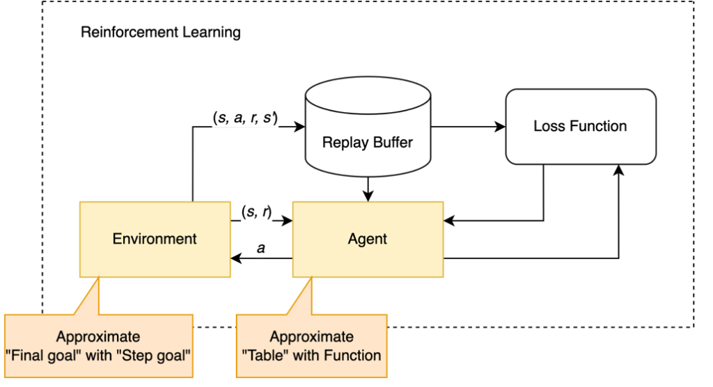
We must first introduce some terminology and define the agents which will learn to trade stocks. In reinforcement learning, agents can be thought of as functions that take in some state, called an observation, and then output an action. Depending on how this action interacts with the environment, they will receive a reward for that action, and update their strategy depending on the strength of the reward. This strategy is called a policy, and is a function that maps observations to actions. This loop, which can be seen in figure 1, repeats to iteratively update the policy and maximize expected rewards.

In this example, we will create two Proximal Policy Optimization (PPO) agents that attempt to outcompete each other, and one PPO agent that acts independently, which will serve as a control. These agents use the PPO neural network as a policy, which was developed by openAI, and is useful in reinforcement learning due to the rate in which they learn/update. These agents could be defined using the Deep Network Designer, although this example defines the networks programmatically. The network architecture for each agent follows:


Environment:
With the agents defined, we must now define the environment, which consists of an observation space, action space, and reward function.
Observation Space:
Our environment consists of 3 stocks simulated via geometric Brownian motion and $20,000 cash. At each time step, each agent sees 19 different values:
- Stocks Owned (3)
- Price Different when Bought (3)
- Cash In Hand (1)
- Price change from yesterday (3)
- % Price change from 2 days ago (3)
- % Price change from 7 days ago (3)
- % Price change from average price of 7 days ago (3)
Action Space:
After receiving a new observation, the agent must make one of 27 possible actions: every combination of entirely buying, entirely selling, and entirely holding for all 3 stocks. For example, (buy, buy, buy), (buy, sell, hold), or (sell, sell, buy).
Reward:
There are two different reward functions at play in this example.
Shared reward for all agents: give the agent +1 as a reward if they made a profit or if they sold stocks while its indicators were suggesting a negative trajectory. Give the agent -1 otherwise. This reward prioritizes making any profit, and can be thought of as “get a reward if you make a profit and get a reward if you avoid losing money”.
Competitive reward for agents 1 and 2: give the agent +0.5 as a reward if it has made more of a profit than its competitor, give the agent -0.5 otherwise.
Given that agent 3 does not contain the competitive reward, a greater performance in agents 1 and 2 would indicate that the competitive strategy aids in learning.
Training:
Now that we have done the heavy lifting and defined our agents and environment, all we need to do is call the train function, specifying the length of each episode to be 2,597 steps, and there to be 2,500 episodes. The results from the agent as shown in the Episode Manager are shown below. As you can see, agents 1 and 2 fight against each other each episode, and this back and forth can be seen in the more jagged nature of their training curves.

Conclusion:
As shown in the results below, agents 1 and 2 outperform agent 3 — their competitive nature aids in learning. Further, agents 1 and 2 over 1.5x their initial $20,000 on the test dataset. These results demonstrate the effectiveness of utilizing competitive agents in financial trading. While the competing agents do not always outperform their solitary counterpart (Agent 3), this work proves the utility and possibility of using this multiagent paradigm!
In the future, this idea could be expanded to many other areas in finance — multiagent reinforcement learning is currently an active area of research, as its competitive nature lends itself well to the inherently competitive world of finance.


댓글
댓글을 남기려면 링크 를 클릭하여 MathWorks 계정에 로그인하거나 계정을 새로 만드십시오.