
Modeling Exchange Rate Volatility
The following post is from William Mueller, Software Developer on the Econometrics Toolbox Team.
Forecasting currency exchange rates is essential to international business management. Doing so successfully is challenging in the era since the collapse of the Bretton Woods agreement on fixed exchange rates (1973), and the introduction of the aggregate Euro currency (1999). Contemporary currency markets are often quite volatile. Economists seek to describe and predict these fluctuations as accurately as possible. This example introduces a basic framework for GARCH modeling of exchange rate volatility.
Retrieve Exchange Rate Data from Haver Analytics®
The Datafeed Toolbox™ enables you to connect to Haver Analytics databases to retrieve their economic data for analysis in MATLAB®.
Connect to the Haver Analytics U.S. Economic Statistics (USECON) database using the haver command.
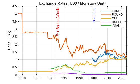
Display the data showing historical monthly prices in U.S. dollars of the Euro, British Pound, Swiss Franc, Indian Rupee, and Chinese Yuan.
figure
plot(dates,Data,LineWidth=1.5)
xline(datetime(1973,3,1),”r-“,”End Bretton Woods”)
xline(datetime(1999,1,1),”b-“,”Start Euro”)
ylabel(“Price (US$)”)
title(“Exchange Rates (US$ / Monetary Unit)”)
legend(series)
grid on

The series exhibit not only pronounced volatility, but volatility clustering during periods of persistently high or low volatility.
Measuring Volatility
A common measure of exchange rate volatility is the sample standard deviation of the percentage daily returns.
Display the volatility for any of the exchange rate series in the period since the introduction of the Euro.
euroEra = (dates >= datetime(1999,1,1));
d = dates(euroEra);
rate =Data(euroEra,2);
returns = 100*diff(log(rate)); % Percentage daily returns
figure
subplot(1,2,1)
h1 = plot(d(2:end),returns); title(“Percentage Daily Returns”);
grid on
subplot(1,2,2)
h2 = histogram(returns); title([“Volatility = “,num2str(std(returns))]);
color = plotcolor(Data,rate,h1,h2); % See supporting code at end of file

The spread of the distribution shows the overall volatility of the currency during the Euro period.
More locally, returns in successive months move up and down and show little autocorrelation.
acf = autocorr(returns);
lag1Autocorrelation = acf(2)
lag1Autocorrelation = 0.2569
However, the magnitude of these movements, measured by squared residuals, shows significant autocorrelation with recent lags.
residuals = returns-mean(returns);
figure
[~,~,~,h] = autocorr(residuals.^2);
set(h(1),Color=color);
title(“Squared Residual Autocorrelation”)

A Ljung-Box Q-test provides a portmanteau statistical test of significance.
[hlbq,pValue,stat,cValue] = lbqtest(residuals.^2)
pValue = 0.0071
stat = 38.7773
cValue = 31.4104
A logical inference of hlbq = 1 is a rejection of the null hypothesis of no significant autocorrelations.
Autocorrelation in the squared residuals indicates volatility clustering.
GARCH Modeling
Common random walk models with innovations of fixed variance are insufficient to capture volatility clustering. GARCH models incorporate an innovations process that is conditional on innovations in previous time periods. As such, they effectively capture the volatility clustering observed in exchange rate series.
Fit a GARCH(1,1) model to the residual returns.
Mdl = garch(1,1);
EstMdl = estimate(Mdl,residuals);
Use the infer function to compute the conditional volatilities of the model.
condVar = infer(EstMdl,residuals);
condVol = sqrt(condVar); % Conditional volatility
figure;
s1 = subplot(2,1,1); s1.Position = [0 0.55 1 0.4];
h1 = plot(d(2:end),residuals,Color=color); title(“Residual Returns”)
grid on
s2 = subplot(2,1,2); s2.Position = [0 0.05 1 0.4];
h2 = plot(d(2:end),condVol,”r”); title(“Conditional Volatility”)
grid on

Peaks in the conditional volatility track clustering in the returns.
Squared standardized residuals exhibit significantly reduced autocorrelation, indicating a good fit.
stdResiduals = residuals./condVol; % Standardized residuals
figure
[~,~,~,h] = autocorr(stdResiduals.^2);
set(h(1),Color=color);

Forecasting
Use the forecast function with the estimated model to compute the minimum mean squared error forecast of the conditional volatility.
horizon = 50; % Forecast horizon
forVar = forecast(EstMdl,horizon,residuals); % Forecast conditional variance
figure
hold on
plot(d(end-100:end),condVar(end-100:end),”r”) % 100 most recent months
plot((d(end)+calmonths(1)):calmonths(1):(d(end)+calmonths(horizon)),forVar,”r–“,LineWidth=1.5);
hold off
title(“Conditional Variance Forecast”)
legend([“Model”,”Forecast”])
grid on

Conclusion
Volatility is only one component of exchange rate models. With data on economic fundamentals of the nations involved in trade, more robust predictive models can be constructed by combining GARCH models with mean models containing relevant exogenous predictors. See Specify Conditional Mean and Variance Models.
References
[1] Granger, C.W. J., and Z. Ding. “Some Properties of Absolute Return: An Alternative Measure of Risk.” Annales d’Économie et de Statistique. No. 40, 1995, pp. 67-91.
[2] Ding, Z., and C.W.J. Granger. “Modeling Volatility Persistence of Speculative Returns: A New Approach.” Journal of Econometrics. Vol. 73, issue 1, 1996, pp. 185-215.
[3] Mandelbrot, B. B. “The Variation of Certain Speculative Prices.” The Journal of Business. Vol. 36, No. 4, 1963, pp. 394-419.
Supporting Code
% Callback for currency selection
function color = plotcolor(Data,rate,h1,h2)
C = colororder;
switch rate(end)
case Data(end,1)
color = C(1,:);
legend(h2,’EURO’,’Location’,’NW’)
case Data(end,2)
color = C(2,:);
legend(h2,’POUND’,’Location’,’NW’)
case Data(end,3)
color = C(3,:);
legend(h2,’CHF’,’Location’,’NW’)
case Data(end,4)
color = C(4,:);
legend(h2,’RUPEE’,’Location’,’NW’)
case Data(end,5)
color = C(5,:);
legend(h2,’YUAN’,’Location’,’NW’)
end
h1.Color = color;
h2.FaceColor = color;
end
- Category:
- Econometrics


Comments
To leave a comment, please click here to sign in to your MathWorks Account or create a new one.