Forecasting workflows often begin with exploration:

• Does a nonlinear approach help?
• How sensitive are results to architecture or training choices?
• How do neural methods compare with classical benchmarks?

The Time Series Modeler app in MATLAB is designed for this early phase. It lets you build, train, and compare time‑series forecasting models—including deep learning approaches—using a guided, visual workflow that complements code‑based analysis.

This post walks through the main steps in the app, alongside the video, so you can follow or revisit each stage at your own pace.

Step 1: Open the Time Series Modeler App

To begin, open MATLAB and launch the Time Series Modeler app from the Apps tab. This opens an interactive environment for building time‑series forecasting models without writing code

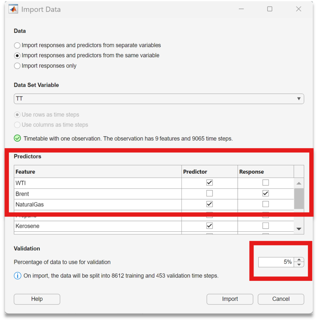
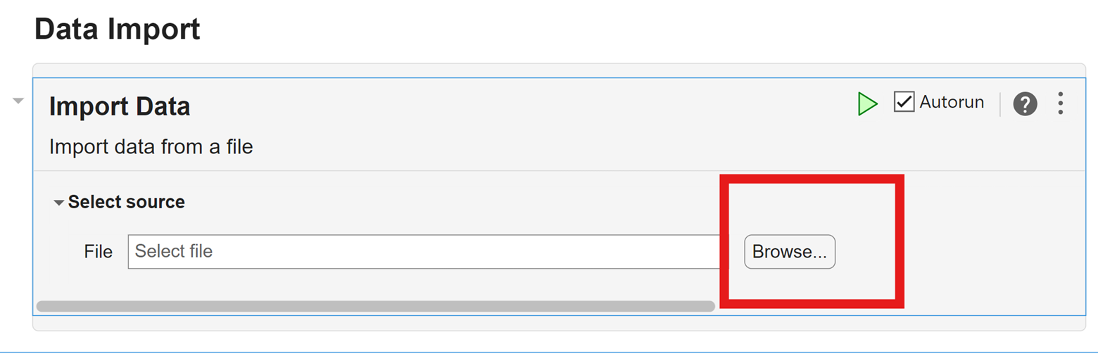
Step 2: Import Time-Series Data

Import your dataset in timetable format. The app automatically detects the time variable and lists the remaining variables for selection.

At this stage you can:

• Select predictors and response variables
• Specify the proportion of data used for validation

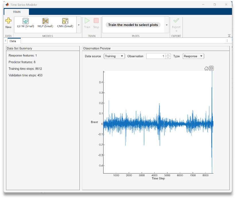
Step 3: Inspect and Explore the Data

After import, the app displays diagnostic plots and summary information so you can explore the data before modeling.

This step is useful for previewing the time-series data, checking observation structure, and getting an early sense of patterns before modeling.

Spending a few moments here can prevent unnecessary retraining later.

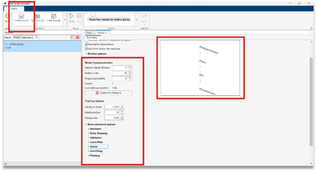
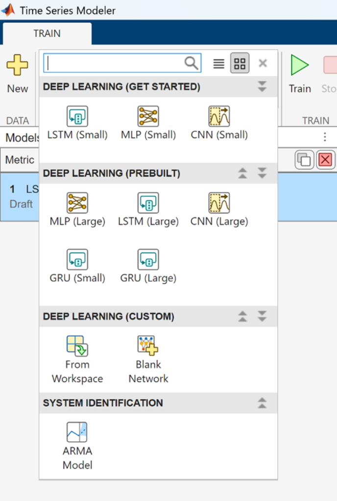
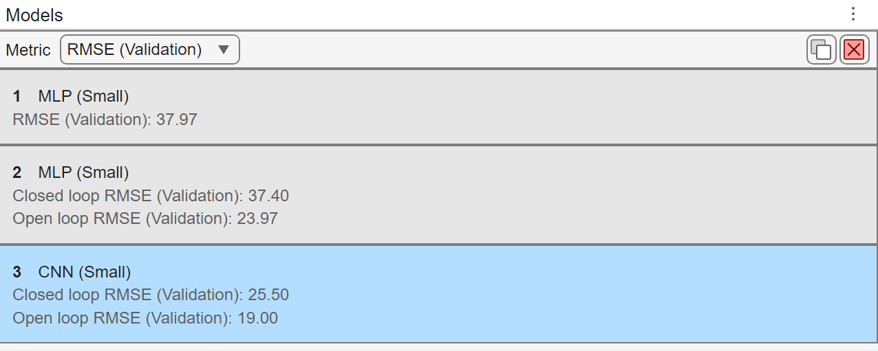
Step 4: Select and Configure a Model

To begin modeling, choose a predefined forecasting model from the Model section.

For example, selecting LSTM (Small) opens a configuration window where you can:

• adjust key hyperparameters
• set training options
• choose solvers and learning rates
• view a diagram of the neural network architecture

The app includes predefined deep learning models such as LSTM, GRU, MLP, and CNN netowkrs, and it also supports ARMA models for comparison when System Identification Toolbox is available.

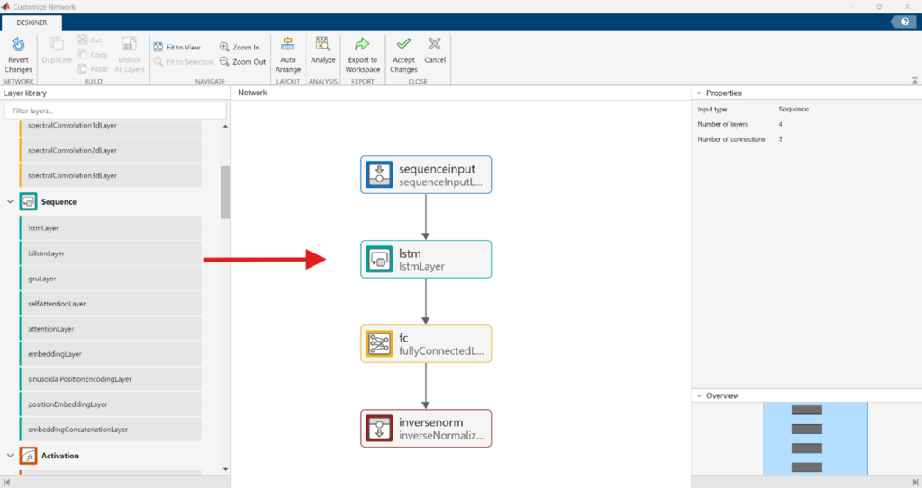
Step 5: Customize the Network (Optional)

If your application requires a more specialized architecture, click Customize Network.

This opens a simplified network editor based on Deep Network Designer, where you can:

• drag and drop layers from the library
• build a custom network structure
• visualize how data flows through the network

This option is useful when experimenting beyond standard templates while still staying within a visual workflow.

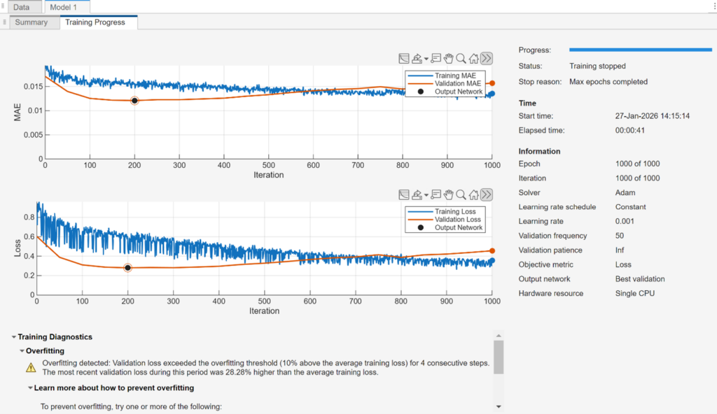
Step 6: Train the model and Review Diagnostics

Click Train to start the training process.

As training progresses, the app displays metrics in real time and provides diagnostic tools to help assess model fit. For example, if signs of overfitting appear, the app surfaces recommendations and configuration options that can help improve generalization.

This makes it easier to iterate on model choices without guessing.

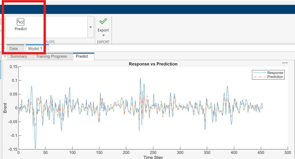
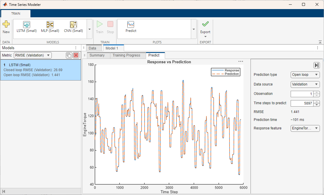
Step 7: Generate Predictions and Evaluate Results

After training completes, click Predict to generate predictions on the training or validation data.

The app compares predicted values with the observed response and displays visual overlays to help you assess accuracy and behavior over time.

This makes it straightforward to evaluate whether a model is capturing key dynamics before moving on.

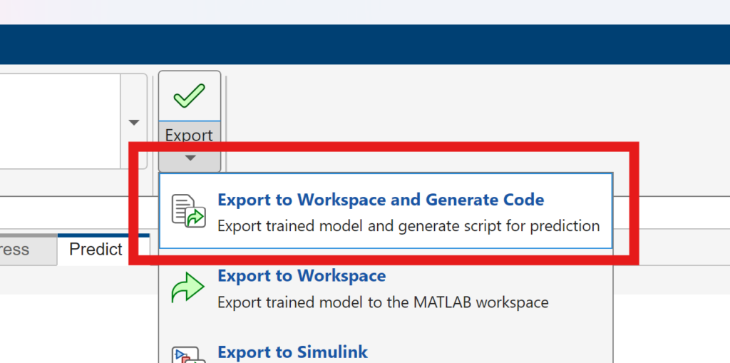
Step 8: Export the Model and Generated Code

When you’re satisfied with the results, use Export to:

• Save the trained model as a struct in the MATLAB workspace
• Export results to the workspace and generate a live script for predicting on new data

This allows you to reproduce results, extend the analysis programmatically, or integrate the model into larger forecasting pipelines.

Summary: A Guided Workflow for Forecasting – No Manual Coding Required

Throughout this workflow, no manual coding is required. The Time Series Modeler app guides you step by step — from data import and exploration, through model configuration, training, diagnostics, and evaluation — using an interactive, visual interface.

As you work, the app automatically generates a live script for prediction on new data when you export. This allows you to reproduce results, extend the analysis programmatically, or integrate the trained model into larger forecasting workflows when needed.

The result is a workflow that supports rapid exploration and comparison early on, while still producing transparent, reusable artifacts for downstream use.

The Time Series Modeler app is included in the Deep Learning Toolbox.

Ready to try it yourself?

• Explore related examples and documentation to go deeper into time-series forecasting with deep learning: Explore Time-Series Forecasting Workflows