
Making even prettier graphs
 |
Guest Writer: Abby Skofield We're excited to welcome Abby Skofield back to the blog! Abby revisits the classic topic of "Making Pretty Graphs"—this time bringing a modern twist with some of the latest MATLAB features. Abby shows how the workflow for customizing and polishing your figures has evolved—making it easier than ever to create beautiful, publication-ready graphics right from your code. For Abby's complete bio, see our Contributors Page. |

Almost 20 years ago, my colleague Jiro Doke published a blog article titled "Making Pretty Graphs," which I re-read and recommend to others more often than I do Jane Austen's collected works. Jiro, this means multiple times a year, believe it or not! In fact, I just shared his blog post with a new colleague today. As much as I love Jiro's original post, we've made some big changes to graphics in the intervening years. I realized that maybe it was time for me to pick up the torch and tackle Jiro's project with the latest version of MATLAB at my fingertips. Today I am going to share with you some examples of how you can use MATLAB code and the properties of our graphics objects to customize the way your MATLAB plots look. You'll probably make different aesthetic choices than I do, but the same techniques can be used to make your MATLAB plots even prettier.
Before joining MathWorks, I worked as a research assistant in a cognitive neuroscience lab, collecting and analyzing experimental data. Like Jiro, I used MATLAB to create data visualizations and, like many customers I've met during my subsequent 12 years at MathWorks, I used other tools to tweak these plots before including them in journal submissions and grant applications. You may yourself be a part of this fellowship, and welcome! If you're a wiz in Illustrator, or just a control freak, this workflow probably suits you pretty well. But perhaps you can save yourself some time the next time around by doing more of these tweaks in MATLAB.
The big benefit of moving this work into MATLAB is that it is scriptable. Any customizations can be captured in code and you can re-run and regenerate the visualization as often as you want while iterating on the final look. And when you're done, you can export it to an image format like PNG, JPG or PDF. Let me show you what I'm talking about!
Create Basic Plot
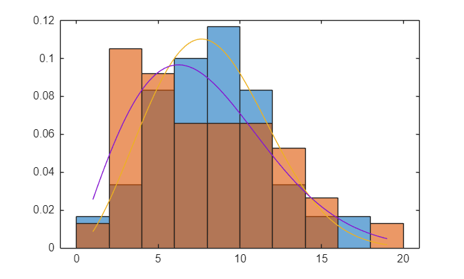
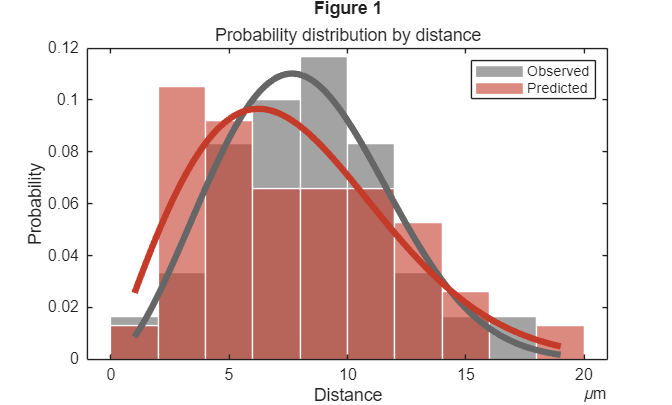
We'll start with some made up data, representing two groups of observed values as well as the results of a probability density estimation for each group of values. We can use histogram to visualize the distribution of values and plot to add in the density curves. What we get is a standard looking axes containing four charts, each of which is given its own color.
[data1, data2, xpdf, pdf1, pdf2] = getFirstDataset;
figure
binEdges = 0:2:20;
h1 = histogram(data1,binEdges,Normalization="pdf",DisplayName="Observed"); % DisplayName stores the legend entry for this plot with the object
hold on
h2 = histogram(data2,binEdges,Normalization="pdf",DisplayName="Predicted");
p1 = plot(xpdf,pdf1);
p2 = plot(xpdf,pdf2);
Adjust Chart Properties
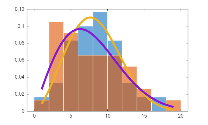
Many customers who share their published figures with us seem to prefer a lighter weight style, with fewer "edges" on their charts. The first thing I will do is clean up the edge lines around the histogram objects by setting the EdgeColor to white. (You can also set most color properties, like EdgeColor, to "none", though in the case of histogram this makes it hard to see where the bin edges are.) I will also bump up the LineWidth of the plot lines to help them stand out. Note that my example demonstrates how you can set a property on a single handle, as with like h1 and h2 below, using the dot-operator to access a property like EdgeColor, or you can set a property on an array of multiple objects, as in [p1 p2] below, using the set command.
h1.EdgeColor = "white";
h2.EdgeColor = "white";
set([p1 p2],LineWidth=4);
SeriesIndex and ColorOrder
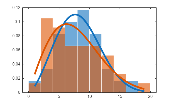
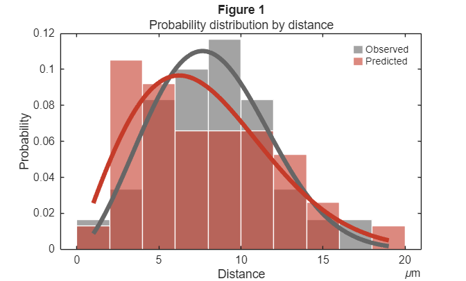
The other thing I've often seen in customers' published examples is a simpler color palette. In my example, I know that each of the density curves should be associated with a different one of the Histogram objects, so I don't need four different colors for the plots. I will use the SeriesIndex property on the plot objects to tell MATLAB to group them, visually, with the respective Histogram. SeriesIndex is how the system indexes into the Axes's ColorOrder palette - charts with the same SeriesIndex value will share the same color.
p1.SeriesIndex = h1.SeriesIndex;
p2.SeriesIndex = h2.SeriesIndex;
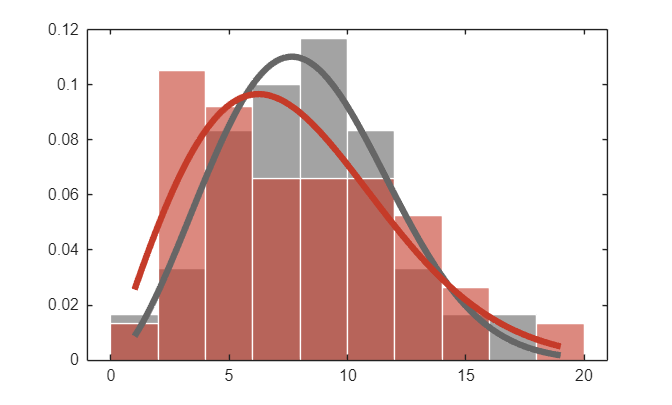
I can then use the colororder function to update the color palette to one that works better for my dataset. Note that hex colors can be easily converted using the hex2rgb function.
redColor = hex2rgb("#C53B29");
greyColor = [0.4 0.4 0.4];
colororder([greyColor;redColor])
Add Labels and Legend
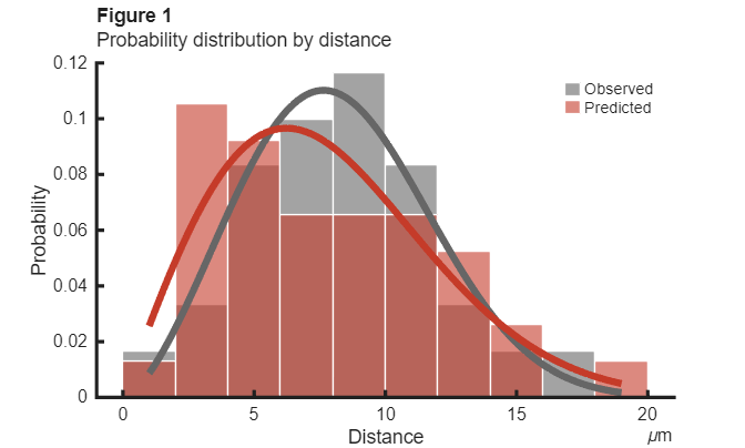
Now that things are starting to look a little more dressed up, it's time to add some labels. Most of the labels you can add to MATLAB plots have their own function, like xlabel or subtitle.
title("Figure 1")
subtitle("Probability distribution by distance")
xlabel("Distance")
ylabel("Probability")
xsecondarylabel("\mum") % Greek and other symbols like mu can be added using TeX markup with a backslash, as in: \mu
By passing in two specific handles to the legend command, I can create a legend with only those two entries. This helps keep things simple since I am only using two distinct colors to differentiate the Observed and Predicted values. Because I specified a DisplayName in each of the histogram commands above, these names will automatically be used in the legend.
leg = legend([h1,h2]);
Most graphics commands, like legend above, optionally return a handle to the object that is created by the command, which enables you to set properties on that object after it is created. In fact, I'll make that legend a little neater and tidier by turning off the Box border and reducing the width used for the legend icons.
leg.Box = "off";
leg.IconColumnWidth = 9;
Adjust Axes and Font Properties
There is one more object we haven't yet tweaked - the Axes. In MATLAB graphics, the Axes object encompasses the x-axis, y-axis and sometimes z-axis which define the space in which the chart objects appear. The Axes object contains multitudes of properties - over 100! So if there's a tweak you're looking for, take a look in our excellent documentation. All graphics objects have documentation pages listing and explaining all of the object's properties, for instance:
- Line properties (plot command): https://www.mathworks.com/help/matlab/ref/matlab.graphics.chart.primitive.line-properties.html
- Axes properties: https://www.mathworks.com/help/matlab/ref/matlab.graphics.axis.axes-properties.html
Of course, you can create an Axes by calling the axes command, but you don't need to - the system creates one automatically when you call a plotting command like histogram or plot. This is what happened in my example, above. If you haven't called axes explicitly and gotten a handle back from this function, you can get a handle to the current Axes using the gca command ("get current axes"). Using this handle, we can set some Axes properties to match the aesthetic applied to the charts.
ax = gca;
ax.Box = "off";
ax.LineWidth = 2;
ax.TitleHorizontalAlignment = "left";
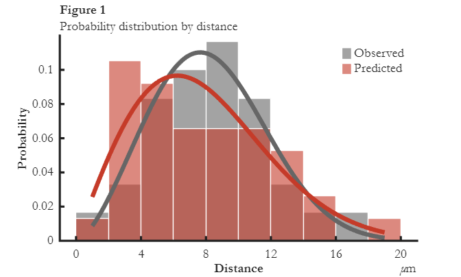
A few final tweaks. I can customize the ticks using the XTick, XTickLabel, and XTickFormat properties on the Axes, or using the xticks and xticklabels commands (same for y and z.)
xticks(0:4:20) % align x-ticks with bin edges
ax.YTick(end) = []; % remove the top y-tick
I didn't grab handles to the x-label or y-label objects when I created them either. I'll use the Axes object's XLabel and YLabel properties to access these Text objects to customize their FontWeights.
ax.XLabel.FontWeight = "bold";
ax.YLabel.FontWeight = "bold";
Many graphics objects have FontSize and FontName properties, and you can customize these individually on each object. However, the fontsize and fontname functions provide a convenient way to specify the same font or font size for all objects in a figure.
fontname("Garamond")
fontsize(12,"points")
Finally, since this is looking so nice, I can use the exportgraphics function to export this figure as an image that can be included in another document. Simply specifying the file extension (e.g. png) along with the desired file name is enough to indicate the output format. You can also, optionally, specify the desired width and height in the units of your choice. I've included the exported image below the Figure here to show the result.
exportgraphics(gcf,"ProbDistrb.png",Width=5,Height=5,Units="inches");

Try another example?
That went so well, I thought I'd try it with a different plot. I'll skip to the good part more quickly this time. Here, you'll see me setting many of the same properties, but this time I'm showing you how you can include the property-sets in the commands themselves as Property-Value pairs.
[xdata, ydata, yerr, fitdata, yfit] = getSecondDataset;
figure
ax = axes(Box = "off",...
LineWidth = 2,...
TitleHorizontalAlignment="left");
ylim([1.5 Inf]) % specifying Inf or -Inf for a limit value uses the auto computed limit
% Turn hold on after creating an axes to assure subsequent plotting
% commands don't reset the properties you've customized.
hold on
barObj = bar(xdata,ydata,...
FaceAlpha = 0.5,...
EdgeColor = "none");
plotObj = plot([0.5 4.5], yfit, LineWidth = 2);
errbarObj = errorbar(xdata,ydata,yerr, ...
LineStyle = "none", ...
Marker = "o",...
MarkerFaceColor = "auto",... % "auto" uses the automatic color, creating a filled look
LineWidth = 2,...
CapSize = 7);
% Remove end ticks after the data is plotted to assure we have the final
% limits.
ax.YTick = ax.YTick(1:(end-1));
ax.XTick = 1:4;
% Specify a colororder and assign the charts the appropriate index into
% this palette of colors.
redColor = hex2rgb("#C53B29");
greyColor = [0.6 0.6 0.6];
colororder([greyColor;redColor]);
barObj.SeriesIndex = 2;
errbarObj.SeriesIndex = 2;
plotObj.SeriesIndex = 1;
legend([errbarObj,plotObj],["mean\pmsd","linear fit"], ...
Location="northwest",...
Box = "off",...
IconColumnWidth = 12);
xlabel("Number of Doses", FontWeight="bold")
ylabel("Concentration", FontWeight="bold")
title("Figure 2","Concentration increases linearly with dose") % quickly create subtitle using the 2nd input argument

I wanted to share one more tip before calling this plot good. You can use the text command to add a Text object somewhere within the Axes as a label. This object is positioned in data units, meaning you'll want to choose an xy-coordinate value that corresponds to available space for an annotation like this. It's helpful to use the HorizontalAlignment and VerticalAlignment properties of the Text object to control where the label appears relative to the anchor point. Note that Text also supports SeriesIndex - by default, Text's SeriesIndex property is set to "none", which is the default black color, but specifying a numeric value can allow you to match Text to plots within the same visualization.
txtObj = text(2.3,3.6,"Slope = "+fitdata(1));
txtObj.FontWeight = "bold";
txtObj.HorizontalAlignment = "right";
txtObj.SeriesIndex = plotObj.SeriesIndex; % to match the fit line
% Oh yeah, and make all the text match our style.
fontname("Garamond")
fontsize(12,"points")

Conclusion
And there you have it! I hope I've given you some new ideas for how to automate the process of generating pretty plots in MATLAB. MATLAB Graphics commands, objects and properties like the ones I shared give you lots of control over the look of your visualizations. I've included a summary of the properties and commands in my examples today at the bottom of the post for reference. What about you? Any other tweaks you find yourself making to your plots? Please share in the comments!
Properties available on many chart objects
- DisplayName
- SeriesIndex
- LineStyle
- LineWidth
- EdgeColor
- FaceAlpha
- Color / FaceColor / MarkerFaceColor
- CapSize (Errorbar only)
Axes properties
- ColorOrder
- Box
- LineWidth
- TitleHorizontalAlignment
- XYZTick, XYZTickLabel
Legend properties
- Box
- Location
- IconColumnWidth
Properties available on many objects containing text
- FontName
- FontWeight
- FontSize
Labeling commands
- title
- subtitle
- x/y/zlabel
- xsecondarylabel
- legend
- xticks, xticklabels
- text
Styling commands
- fontsize
- fontname
- colororder
function [dist1, dist2, xgrid, pdfEst1, pdfEst2] = getFirstDataset
% first data set
dist1 = [ 6.2 10.1 9.3 8.1 8.8 7.1 7.8 5.9 7.3 8.2 ...
16.1 12.8 9.8 11.3 5.1 10.8 7.7 7.7 1.2 8.3 2.3 ...
4.3 2.9 14.8 4.6 12.8 9.8 11.3 5.1 10.8]';
dist2 = [ 3.1 13.6 14.5 5.2 5.7 5.2 5.7 6.5 6.4 3.5 11.4 9.3 12.4 ...
5.3 6.4 3.5 11.4 11.4 11.4 9.3 12.4 18.3 15.9 4.0 4.0 10.4 ...
8.7 3.0 3.0 12.1 3.9 6.5 3.4 3.4 8.5 0.9 9.9 7.9 ]';
pd1 = fitdist(dist1,"Weibull");
pd2 = fitdist(dist2,"Weibull");
xgrid = linspace(1,19,100)';
pdfEst1 = pdf(pd1,xgrid);
pdfEst2 = pdf(pd2,xgrid);
end
function [xdata, ydata, yerr, fitdata, yfit] = getSecondDataset
% second data set
xdata = 1:4;
ydata = [2.11 3.12 3.97 4.56];
yerr = [0.25 0.21 0.37 0.51];
fitdata = polyfit(xdata,ydata,1);
yfit = fitdata(1)*([0.5 4.5]) + fitdata(2);
end


Comments
To leave a comment, please click here to sign in to your MathWorks Account or create a new one.