
On The Edge
In an earlier post, we discussed how the contour functions interpolate between values. Another important issue is how the contour functions deal with contour levels which are exactly the same as values in the input data. Some users are often surprised by what happens in this case because there are some subtle issues involved. Let's take a detailed look.
Contents
We'll start with a simple matrix with 3 different values.
z=zeros(6);
z(2:3,2:3)=-1;
z(4:5,4:5)=1;
We'll also want the following helpful function to label the values of our matrix.
type labelcontourvalues
function labelcontourvalues(z)
    for r=1:size(z,1)
        for c=1:size(z,2)
            v = z(r,c);
            color = 'black';
            if (v < 0)
                color = 'blue';
            elseif (v > 0)
                color = 'red';
            end
            h = text(c,r,num2str(v));
            h.HorizontalAlignment = 'center';
            h.VerticalAlignment = 'middle';
            h.Color = color;
            h.BackgroundColor = 'white';
            h.FontSize = 8;
            h.Margin = eps;
        end
    end
end
Contours
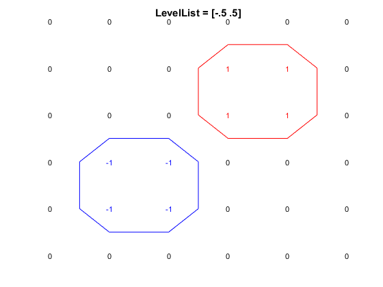
If we create a contour with levels which are in between those values, then it's pretty straightforward. Each contour line separates two areas which are above and below the value of the contour line.
contour(z,'LevelList',[-.5 .5]);
colormap([0 0 1;1 0 0]);
caxis([-1 1]);
axis off
labelcontourvalues(z)
title('LevelList = [-.5 .5]')
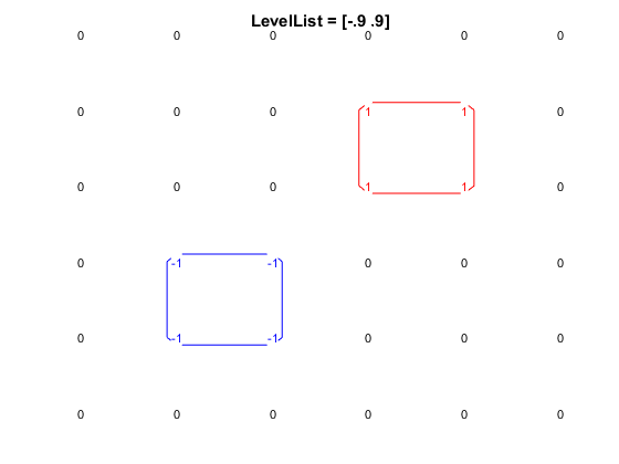
And if we move the levels very close to the values, those two contour lines move closer to the points.
contour(z,'LevelList',[-.9 .9]);
axis off
labelcontourvalues(z)
title('LevelList = [-.9 .9]')
But when the levels are exactly equal to data values, we get a somewhat surprising result.
contour(z,'LevelList',[-1 1]);
axis off
labelcontourvalues(z)
title('LevelList = [-1 1]')
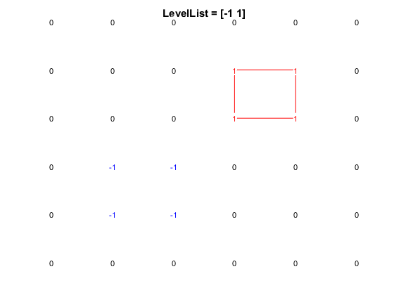
In this case, contour has drawn a line for the level 1. It goes right through the 1 values, as we'd expect. But it didn't draw a line for the level -1. It seems like drawing the -1 level would make this more symmetric, doesn't it?
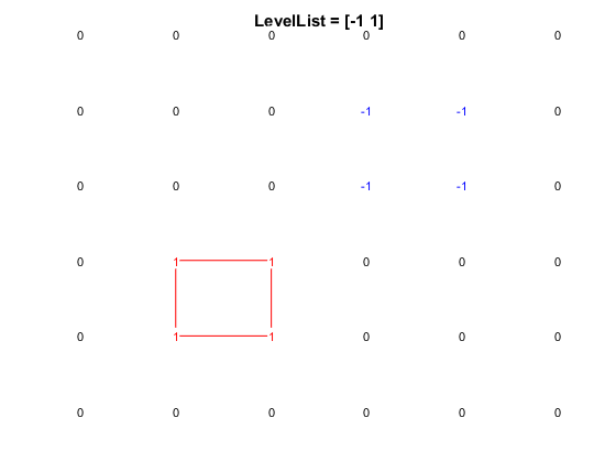
And furthermore, if flip the sign, we get a different picture. That also seems surprising, doesn't it?
cla
minus_z = -z;
contour(minus_z,'LevelList',[-1 1])
axis off
labelcontourvalues(minus_z);
title('LevelList = [-1 1]')
Well things really aren't symmetric here. We can see that if we add a level at 0.
contour(z,'LevelList',[-1 0 1]);
colormap([0 0 1;0 0 0;1 0 0]);
caxis([-1 1]);
axis off
labelcontourvalues(z)
title('LevelList = [-1 0 1]')
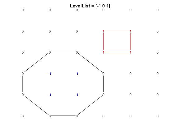
Notice how the 0 level goes through the 0 values which have neighboring -1 values, but it doesn't go through the 0 values which are next to 1 values.
It's hard to come up with a contour algorithm which would really be symmetric in this case. Would it somehow go through the middle of the region that is all 0's? You could try that, but it turns out that there are some nasty surprises down that path because of all of the special cases. You could also try drawing a curve on each side of that region of 0's, but that'd be rather strange too. Some people have proposed that contour should fill the region of 0's, but if you try that, you'll see that it looks pretty ugly.
So contour needs to go around one side of the area that is exactly equal to the level. It does this by following a simple rule. It draws a line which separates regions which are less than the level from regions which are greater than or equal to the level.
This is why it doesn't draw a curve for the -1 level. There are no values which are less than -1, so there is no area which should be separated from the area which is equal to -1.
Filled Contours
If we use the contourf function, then we'll get filled polygons instead of lines. If we do, we'll see that we get the same curves for the levels 0 and 1 as we did with contour.
We also get a blue region for the values (v >= -1 & v < 0), a white region for the values (v >= 0 & v < 1), and a red region for the values (v >= 1).
contourf(z,'LevelList',[-1 0 1]);
colormap([0 0 1;1 1 1;1 0 0]);
caxis([-1 1]);
axis off
labelcontourvalues(z)
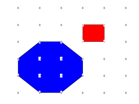
Notice that it didn't draw a square around the -1 values. This is consistent with what the contour function did. But MATLAB has historically had some inconsistencies between the rules used by the different contour functions. In R2014b we made them all use the same rule.
Well, actually there is still an inconsistency in MATLAB's contour functions; that is if we consider isosurface a contour function.
The isosurface function is the 3D analogue of contour. It takes a 3D array, instead of a 2D array, and it draws the surface which separates regions, rather than a curve.
We can recreate our example in 3D and see what isosurface does with it.
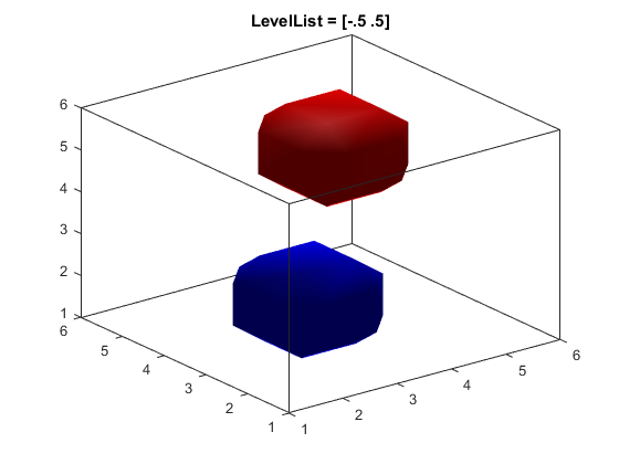
If we isosurface at -1/2 and 1/2, we get two surfaces, just like the two curves we got when we used those levels for contour.
z=zeros([6 6 6]);
z(2:3,2:3,2:3)=-1;
z(4:5,4:5,4:5)=1;

cla
isosurface(z,-.5)
isosurface(z,.5)
title('LevelList = [-.5 .5]')
xlim([1 6])
ylim([1 6])
zlim([1 6])
camlight
axis on
view(3)
But if we isosurface at -1 and 1, we only get one. The problem is that it's the blue one, while contour gave us the red one.
cla
isosurface(z,-1)
isosurface(z,1)
title('LevelList = [-1 1]')
camlight
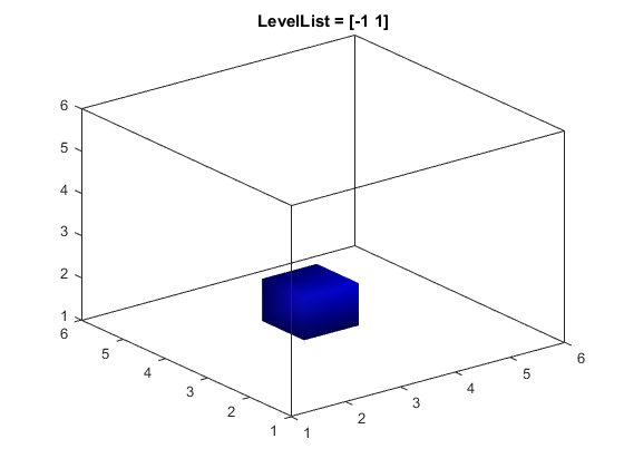
It turns out that isosurface uses the opposite rule from contour. It draws a surface between regions which are less than or equal to the level and regions which are greater than the level.
In early versions of MATLAB, there wasn't much consistency between these functions. We've now got the 2D contour functions consistent with each other, but we haven't yet changed isosurface to match.
- 类别:
- Geometry

