
Quantum computing in MATLAB R2023b: On the desktop and in the cloud
Back in May of this year i attended the ISC High Performance Computing conference with a few other colleagues from MathWorks and was astonished at the number of booths related to various quantum computing intitiatives. I had more conversations about quantum computing in those few days than I'd had in years leading up to the event! As such, it seems rather timely that it's now possible to do quantum computing in MATLAB.
Getting started with quantum computing in MATLAB
The MATLAB Support Package for Quantum Computing is a free add-on developed by MathWorks. There are several ways to install it but my preferred way is via the Add-on Explorer.
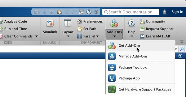
Once in Add-on explorer, just search for quantum computing and you'll find it. Another way to get it is via its entry on File Exchange. Quantum computing has been available in MATLAB for a while now -- since R2023a but it recently got a few additional updates so now is a good time to dive in.
MATLAB currently supports a flavour of quantum computing called gate-based quantum computing at the root of which is a so-called quantum circuit. Let's create and visualise one
gates = [hGate(1);
cxGate(1,2);
cxGate(1,3)];
C = quantumCircuit(gates);
plot(C)

This is a three-qubit circuit with three quantum gates. Each horizonal line in the plot represents one of the qubits and the gates are arranged from left to right in the order that they are applied. The first qubit has a Hadamard gate applied to it while CNOT gates have been applied to the second and third qubits, using the first qubit as the control.
In order to actually run this quantum circuit, you'd need access to a real quantum computer and these are not the sort of thing that one has on their desk!
For now, let's simulate this circuit, specifying that each qubit has an inital state of (never seen this notation before? It's an example of bra-ket notation) . We'll discuss how to run it on a real quantum computer later.
S = simulate(C,"000")
Let's express the simulated quantum state as a formula
f = formula(S)
There are two possible quantum states in this system but if you were were to actually observe it, you'd only see one. Which one you'd see is a matter of chance which is one of the consequences of quantum mechanics. Let's ask MATLAB for the possible states and the probabilities of seeing each one.
[states,P] = querystates(S)
Each state has a 50% change of being measured. We can plot this as a histogram but it's not a particularly interesting one
histogram(S)

If you actually had that quantum system, you'd not be able to directly measure probabilities. What you'd measure are the states and you'd do it a bunch of times to get an approximation of the probabilities. How do you do that in MATLAB?
% Simulate 50 quantum measurements of the circuit
M = randsample(S,100)
Put the result into a table
simT = table(M.Counts,M.MeasuredStates,VariableNames=["Counts","States"])
This is roughly what you'd expect if the probability of getting each state is 50%. Anyone expecting exactly 50 Counts for each state should retake probability-101!
Qubits? Gates? Quantum probabilities? What's going on?

I've shown you how to create and simulate a quantum circuit in MATLAB but, at this point, you may be wondering what on earth is going on? How does any of this relate to implementing numerical algorithms? This talk of qubits, gates and state probabilities is rather far removed from the variables, if-statements and for-loops that I used when I first studied how to solve problems. As Alice famously said "Toto, I’ve a feeling we’re not in Kansas anymore"
Quantum computing is a totally different way of approaching computation that requires rather more explanation than I could fit into a blog post. We've got you covered, however. If you are totally new to the field of quantum computing, just start with this article in the MATLAB documentation: Introduction to Quantum Computing. You may also find this MathWorks quantum computing cheat sheet useful.
Another article that you may find interesting is this in-depth one from fellow MathWorks blogger Sofia Ma: Quantum Computing for Optimizing Investment Portfolios
An insight that really helped me make my first baby steps into quantum computing is to understand that the states of quantum systems can be represented by vectors while all of the gates have matrix representations. Here are two of them. For more, see Types of Quantum Gates
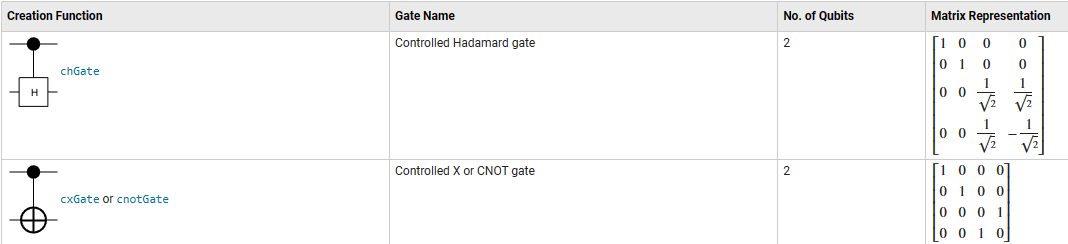
or in other words....

If you have any other favourite sources for learning about quantum computing, let me know in the comments section.
Applications of quantum computing
Maybe you don't care so much about how to design a quantum algorithm and want to jump straight to potential applications. MathWorks has you covered here as well with a range of algorithms fully implemented in the new framework and available in the documentation. These include
- Graph Coloring with Grover's Algorithm
- Ground-State Protein Folding Using Variational Quantum Eigensolver (VQE)
- Quantum Monte Carlo (QMC) simulation
We also have a set of open-source examples of quantum computing algorithms over on GitHub covering topics such as Portfolio Optimisation and Machine Learning classifiers. Pull Requests are welcome!

We've also implemented something called QUBO -- Quadratic Unconstrained Binary Optimization which can be used to solve combinatorical optimization problems such as the Traveling Salesperson Problem and the Capacitated Vehicle Routing Problem among others.
Quantum computing has the potential to revolutionise how we solve many problems that are difficult using conventional computers. That is, problems that would take a conventional supercomputer years to solve could be solved very quickly using a quantum algorithm on a suitable quantum computer. This is why there is so much hype around the subject and why there are so many quantum computing booths at supercomputing conferences.
Unfortunately, the quantum computers that currently exist are not yet powerful enough to do this and thus, revolutionise computing.
Quantum computers do exist, however, and they are good enough for us to test that our simulated algorithms do actually work on real quantum hardware...even if they are not yet quite good enough to give your local supercomputer a run for its money.
Running MATLAB quantum algorithms on real quantum computers using Amazon AWS
Real quantum computers are rather difficult to buy and it's unlikely that you have one sitting on your desk. An organisation who can give you access to some, however, is Amazon AWS and they make them available to the world via the Amazon Braket service. Details on how to connect MATLAB with the Amazon Braket service are at Run Quantum Circuit on Hardware Using AWS - MATLAB & Simulink (mathworks.com)
Before running this code, I had to create an S3 bucket with a name that started with the string "amazon-braket-". You'll need to create your own unique bucket name in your AWS account. Details on how to create S3 buckets in MATLAB can be found at Transfer Data to Amazon S3 Buckets and Access Data Using MATLAB Datastore - MATLAB & Simulink (mathworks.com)
There are two types of quantum resource available on Amazon that are of interest to us
- QPU Devices: These devices are quantum computers used to perform probabilistic measurements of circuits. Not all QPU devices are supported. To find out if a device is supported, try connecting to the device using quantum.backend.QuantumDeviceAWS. Availability and number of qubits supported can also vary, so check the device details before sending circuits for measurement.
- Simulator Devices: Because memory usage scales exponentially with the number of qubits, larger circuits with many qubits might stretch the limits of memory available on your local computer. To address that issue, AWS also provides cloud-scale simulators. The functionality is similar to using randsample on your local system, but the simulators can support up to 34 qubits with cloud-scale performance.
At the time of writing, the example in MathWorks documentation connects to a simulator: "SV1", a state-vector simulator used for prototyping circuits.
I want to run on the real-deal though! I can't say I've done quantum computing until I've submitted a job to a real quatum computer. I took a look at the available devices on Amazon Braket and randomly chose the Rigetti Aspen-M-3. This is a 79 Qubit device and the details section over at Amazon told me that "Rigetti quantum processors are universal, gate-model machines based on tunable superconducting qubits." Sounds cool! Superconductors and programmable quantum computers! If only 1996 physics undergraduate Mike Croucher could see me now 🙂
% This code will not work for you unless you have configured AWS correctly
reg = "us-west-1";
bucketPath = "s3://amazon-braket-walkingrandomlyblog/default"; % You'll need to change this name to your own bucket
device = quantum.backend.QuantumDeviceAWS("Aspen-M-3",Region=reg,S3Path=bucketPath)
The fetchDetails command can be used to....um...fetch the details of the quantum device I want to submit jobs to.
fetchDetails(device)
I'm connected and I'm ready to go. Remember that circuit that I created at the beginning of the blog post?
plot(C)
I've simulated it on my desktop. Time to run it on the real thing in the cloud using the run command
task = run(C,device)
I'm in the quantum queue in the cloud! Let's get MATLAB to wait until the task is finished. The following command blocks execution until the task on the quantum device has finished running.
wait(task)
Eventually, the task will complete and I can get the results
R = fetchOutput(task)
Results from running on a real quantum computer
When I simulated this quantum circuit on my local machine 100 times, I got the following results
simT
Running the circuit on a real system gave the following
T = table(R.Counts,R.MeasuredStates,VariableNames=["Counts","States"])
The overall number of Counts sum to 100 because that's the default number of times the run command runs the circuit. Each of these runs is called a shot.
histogram(R)

What's interesting here is that along with the two states I expected to observe, I've also observed every other possible state a small number of times. I understand that this is due to noise in the system. Real quantum computers are not perfect devices and this noise is part of the reality of working with quantum algorithms on real devices.
It's difficult to convey to you how exciting this feels! I know that the computation I've done is essentially a pointless demo that I've lifted from the MATLAB documentation but there is just something thrilling about running code on a completely different type of computer to anything I've ever used before.
The run you see above is the first (and so far only) time I have ever run anything on a real quantum computer!
Costs of the AWS quantum computation
As you might expect, running jobs on a quantum computer in the cloud costs money. The way Quantum jobs are currently priced by AWS are a cost per task and an additional cost per shot.
In the context of this calculation, you can think of the task as setting up the circuit and each shot as the cost of running that circuit 1 time. At the time of writing, the device I used had a cost of 30 cents per task and 0.035 cents per shot so the 100 shot calculation cost me about $0.34. There will also be S3 storage costs but for this computation I'm guessing it will be pretty negligible. I doubt I'll be sufficiently motivated to fill in my expense claim to MathWorks for cloud costs associated with this blog post.
Version of the MATLAB Support Package for Quantum Computing used
I used version 23.2 of the MATLAB Support Package for Quantum Computing. You can see which one you have installed by executing
matlabshared.supportpkg.getInstalled
- Category:
- linear algebra,
- New Features,
- quantum computing


Comments
To leave a comment, please click here to sign in to your MathWorks Account or create a new one.