Faster Ordinary Differential Equations (ODEs) solvers and Sensitivity Analysis of Parameters: Introducing SUNDIALS support in MATLAB

著者 Mike Croucher, April 17, 2024

1598 ビュー (過去 30 日間) | 0 いいね | 2 コメント

Late last year I introduced the new solution framework for solving Ordinary Differential Equations (ODEs) that made its debut in MATLAB R2023b. I demonstrated how it allowed users to do all kinds of things much more easily than before but stressed that the R2023b release was mostly about the new interface. I told you "There are no new solvers or any fundamentally new functionality....yet!". A few people picked up on the 'yet', correctly guessing that there would be new solvers and functionality soon. In R2024a, we've made a start on this by adding support for some of the SUNDIALS solvers.

What is SUNDIALS?

SUNDIALS is a SUite of Nonlinear and DIfferential/ALgebraic equation Solvers, an award-winning set of open source ODE solvers from Lawrence Livermore National Labs. Functionality from SUNDIALS has been available via Simbiology for a while and now we've brought it to all MATLAB users via the new ODE solver interface. There are several solvers in the SUNDIALS suite and we've added support for three of them via new values of the Solver property of the ode class: "cvodesstiff", "cvodesnonstiff" and "idas".

"cvodesnonstiff" Variable-step, variable-order (VSVO) solver using Adams-Moulton formulas, with the order varying between 1 and 12. See CVODE and CVODES.
"cvodesstiff" Variable-step, variable-order (VSVO) solver using Backward Differentiation Formulas (BDFs) in fixed-leading coefficient form, with order varying between 1 and 5. See CVODE and CVODES.
"idas" Variable-order, variable-coefficient solver using Backward Differentiation Formulas (BDFs) in fixed-leading coefficient form, with order varying between 1 and 5. See IDA and IDAS.

An example: How to switch to a SUNDIALS solver in MATLAB

Let's begin by solving the classic predator-prey equations

dxdt=p1x-p2xydydt=-p3y+p4xy

with parameters p1=0.4,p2=0.4,p3=0.09,p1=0.1and initial conditions x(0)=1,y(0)=1

Setting up and solving the problem using the ode class looks like this

d = ode(ODEFcn=@(t,y,p) [p(1)*y(1) - p(2)*y(1)*y(2); ...

                           p(3)*y(1)*y(2) - p(4)*y(2)]);

% Set initial conditions and parameters

d.InitialTime = 0;

d.InitialValue = [1;1];

d.Parameters = [.4 .4 .09 .1];

% Set the relative tolerance

d.RelativeTolerance = 1e-6;

At this point, I could just get on and solve the system of ODEs with the solve function and MATLAB would attempt to choose a suitable solver for me and in R2024a it happens to choose ode45 for this problem. This could change in future versions though so let's explicitly choose ode45 so we know exactly what we'll be using.

% Select the ode45 solver

d.Solver = "ode45";

% Solve over a short time span

sol = solve(d,0,100);

plot(sol.Time,sol.Solution,LineWidth=2)

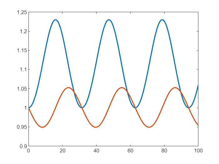
To switch to using the non stiff version of SUNDIAL's CVODES solver, I just need to do

% select the cvodesnonstiff solver

d.Solver = "cvodesnonstiff";

and then solve as before

% Solve over a short time span

sol = solve(d,0,100);

plot(sol.Time,sol.Solution,LineWidth=2)

Not much appears to have changed! So what are the benefits of using the SUNDIALS solvers?

SUNDIALS solvers can lead to improved performance

The first potential benefit of the new SUNDIALS solvers is performance. I'm going to switch back to ode45, solve over a much larger time span and use the timeit function to get solution time

d.Solver = "ode45";

timeOde45Fcn = @() solve(d,0,15000);

ode45Time = timeit(timeOde45Fcn)

ode45Time = 0.0828

Now let's solve the exact same problem with SUNDIALS' CVODES non stiff solver.

d.Solver = "cvodesnonstiff";

timeCvodesFcn = @() solve(d,0,15000);

cvodesTime = timeit(timeCvodesFcn)

cvodesTime = 0.0214

Let's see what the speed-up is

fprintf("The SUNDIALS solver cvodesnonstiff is %f times faster than ode45 for this problem\n",ode45Time/cvodesTime)

The SUNDIALS solver cvodesnonstiff is 3.861154 times faster than ode45 for this problem

I was pretty pleased with this! Internal presentations about the new solver suggested that the speed-up would be ~2x or so for most benchmarks and I've gotten way more than that here. The reasons for the speed-up of cvodesnonstiff compared to ode45 are primarily that it requires fewer steps and its slightly faster per step. The SUNDIALS suite is written in C and we've also performed some JIT magic to reduce the overhead of calling a MATLAB function from a C++ function.

We can get some insight into this by looking at the solutions. Over the time span [0,15000], ode45 takes 33409 steps for the tolerance I have set

d.Solver = "ode45";

ode45Sol = solve(d,0,15000)

ode45Sol = 
  ODEResults with properties:

        Time: [0 0.4988 0.9975 1.4963 1.9951 2.4938 2.9926 3.4913 3.9901 4.4904 4.9906 5.4909 5.9911 6.4790 6.9668 7.4546 7.9425 8.3974 8.8523 9.3072 9.7621 10.1966 10.6312 11.0657 11.5003 11.9240 12.3477 12.7714 13.1950 13.6168 … ] (1×33409 double)
    Solution: [2×33409 double]

while cvodesnonstiff takes 11503 steps

d.Solver = "cvodesnonstiff";

cvodesSol = solve(d,0,15000)

cvodesSol = 
  ODEResults with properties:

        Time: [0 0.0188 0.0376 0.0903 0.1430 0.3933 0.7597 1.1260 1.7017 2.2774 3.0827 3.8880 5.1824 6.4767 7.7711 9.0655 10.3599 11.2558 12.1516 13.0475 13.9434 14.8392 15.7351 16.6309 17.5268 18.4226 19.3185 20.2144 21.1102 22.0061 … ] (1×11503 double)
    Solution: [2×11503 double]

That's 2.9x fewer steps than ode45 but there's more than a 2.9x speed-up so the speed-difference is clearly not just because the new solver requires fewer steps. 

I've been comparing against ode45 because that's the algorithm I always reach for first. However, cvodesnonstiff is most similar to ode113 as far as the algorithm under the hood is concerned and it turns out that ode113 requires about the same number of steps as cvodesnonstiff.

d.Solver = "ode113";

ode45Sol = solve(d,0,15000)

ode45Sol = 
  ODEResults with properties:

        Time: [0 0.0125 0.0250 0.0500 0.1000 0.2000 0.4000 0.6000 0.8000 1.2000 1.6000 2.0000 2.4000 3.2000 4.0000 4.8000 5.6000 6.4000 8.0000 9.3769 10.6161 11.7314 12.8467 13.9620 15.0773 16.1926 17.3079 18.4232 19.5385 20.6538 … ] (1×11766 double)
    Solution: [2×11766 double]

Very close in terms of number of steps but it turns out that ode113 is even slower than ode45 for this problem

d.Solver = "ode113";

timeOde113Fcn = @() solve(d,0,15000);

timeOde113 = timeit(timeOde113Fcn)

timeOde113 = 0.1106

fprintf("The SUNDIALS solver cvodesnonstiff is %f times faster than ode113 for this problem\n",timeOde113/cvodesTime)

The SUNDIALS solver cvodesnonstiff is 5.162407 times faster than ode113 for this problem

When I spoke to development about these speed differences they told me that I happened to choose a problem that really allows the new SUNDIALS integration to shine! For example, I chose an integration time that was large enough to dwarf the startup cost. For various reasons, the overhead for getting from ode object into the SUNDIALS solver is generally bigger than getting into ode45 and friends. Once we are in SUNDIALS, however, things can really fly for small problems like this.

For bigger, stiff problems, we find less of a performance difference between the MATLAB and SUNDIALS solvers. The way this was explained to me is to consider what the solver actually does. It evaluates a function handle and then does some vector-vector or matrix-vector operations/solves/etc. When the problems get big, the linear algebra starts to dominate and the time per step will be similar for both solvers. At this point, the winning solver is the one that happens to have fewer steps or which one that manages to trigger fewer matrix factorizations etc, which again, is problem dependent. 

So, the SUNDIALS can be a lot faster than ode45 and friends...and sometimes its not. The exact speed difference between solvers depends heavily on the problem and I encourage you to investigate on your own problems and let me know what you find.

SUNDIALS solvers allow sensitivity analysis of parameters in systems of ODEs

Having a faster ODE solver in MATLAB is great but there is another reason to love the SUNDIALS integration: Sensitivity analysis of parameters. This is functionality that Simbiology users have had for a while but now some of it is in MATLAB itself. Sensitivity analysis examines how changes in parameter values can affect the solution of the ODE system. 

The MATLAB documentation demonstrates this by looking at a Sensitivity analysis of a SIR epidemic model so I went looking for a different model to play with. I soon found the CARRGO model [1] via a paper about methods for assessing sensitivity in biological models [2]. It models the interaction of cancer cells and CAR T-cells which are used to destroy them and is a variation of Lotka-Volterra predator-prey equations. The system of ODEs is 

dxdt=ρx(1-xγ)-κ1xydydt=κ2xy-θy

x is the density of cancer cells andy is the density of CAR T-cells. In MATLAB, I'll refer to the parameters as a vector p and since there are 5 parameters here, we'll have a 5 element vector. The meaning of each parameter and the number I'll give it in MATLAB is as follows

$κ_{1}$ = p(1): The killing rate of the CAR T-cells.
$κ_{2}$ = p(2): Net rate of proliferation of CAR T-cells
θ= p(3): Death rate of CAR T-cells
ρ= p(4): Net growth rate of cancer cells
γ= p(5): Cancer cell carrying capacity

Sensitivity analysis will give us the derivatives of x(density of cancer cells) and y(density of CAR T-cells) with respect to these five parameters.

Setting the equations up in MATLAB:

F = ode();

F.ODEFcn = @(t,x,p) [ p(4) * x(1) * (1-x(1) / p(5))-p(1) * x(1) * x(2); p(2)* x(1) * x(2)-p(3) * x(2)];

Sahoo et al [1] fitted this model to empirical data (Using MATLAB and fmincon so the paper tells us) and found the following parameters and initial values

F.InitialValue = [1.25*10^4 , 6.25*10^2];

F.Parameters = [6*10^-9, 3*10^-11, 1*10^-6, 6*10^-2, 1*10^9];

Set the solver to cvodesnonstiff and we can get the solution to the system of equations as usual

F.Solver = "cvodesnonstiff";

sol = solve(F,0,1000)

sol = 
  ODEResults with properties:

        Time: [0 0.4432 0.8865 1.8492 2.8119 5.1685 10.1265 15.0845 20.0425 25.0005 29.9585 34.9165 39.8745 44.8326 49.7906 54.7486 59.7066 64.6646 69.6226 74.5806 79.5386 84.4967 89.4547 94.4127 99.3707 104.3287 109.2867 114.2447 … ] (1×112 double)
    Solution: [2×112 double]

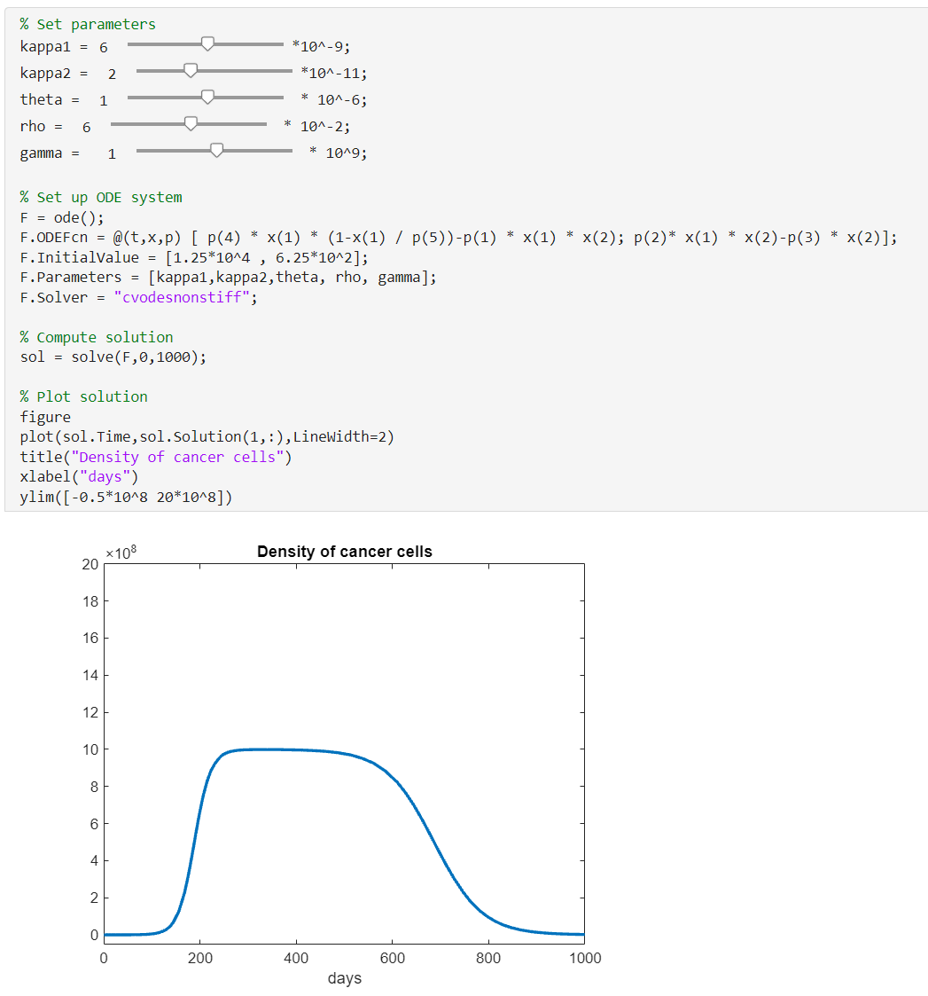
Next, I plot these solutions

tiledlayout(2,1)

nexttile

plot(sol.Time,sol.Solution(1,:),LineWidth=2)

title("x : density of cancer cells")

xlabel("days")

ylim([-0.5*10^8 11*10^8])

nexttile

plot(sol.Time,sol.Solution(2,:),LineWidth=2)

title("y : density of CAR T-cells")

xlabel("days")

ylim([-0.5*10^6 16*10^6])

sgtitle("Solutions of the CARRGO system of ODEs")

Computing the parameter sensitivities

Computing the sensitivities of the system of equations to all 5 parameters is very easy. We simply add the following to the ODE object.

F.Sensitivity = odeSensitivity();

and run the solve command as before. 

sol = solve(F,0,1000)

sol = 
  ODEResults with properties:

           Time: [0 1.6859e-12 1.6860e-08 1.8545e-07 1.8713e-06 1.8730e-05 5.4218e-05 4.0909e-04 0.0032 0.0060 0.0145 0.0229 0.0539 0.1077 0.2072 0.4305 0.6539 0.9892 1.6542 2.3193 3.5475 4.7757 6.0039 8.2478 10.4918 12.7357 14.9797 … ] (1×225 double)
       Solution: [2×225 double]
    Sensitivity: [2×5×225 double]

Note that this time, our ODEResults has a Sensitivity field alongside the Solution. There are 2 x 5 sets of Sensitivity results corresponding to the partial derivatives of either of our 2 variables with respect to the 5 parameters. If I wanted to only consider a few indices, I would change ParameterIndices accordingly.

You're going to need to squeeze!

Let's get the result for the first variable, x, and the first parameter, κ1, i.e. ∂x∂κ1

dXdKappa1 = sol.Sensitivity(1,1,:);

sensitivitySize = size(dXdKappa1)

sensitivitySize = 1×3
     1     1   225

The problem with this is that it is a 1 x 1 x 225 array so plotting it directly won't work!

plot(sol.Time,dXdKappa1)

Error using plot
Data cannot have more than 2 dimensions.

You have to first squeeze it to get rid of the redundant singleton dimension. You'll find that there is a lot of squeezing to be done when dealing with sensitivities! 

figure

plot(sol.Time,squeeze(dXdKappa1),LineWidth=2)

ylabel("$\frac{\partial x}{\partial\kappa_1}$",Interpreter="latex")

xlabel("days");

title("Sensitivity of Cancer Cells in the CARGGO Model to the $\kappa_1$ parameter",Interpreter="latex")

The result is the partial derivative of x with respect to the parameter κ1

Normalizing and comparing the sensitivity functions

The epidemic example in the MATLAB documentation for Sensitivity Analysis tells us that sensitivity functions are often normalized such that the result describes the approximate percentage change in each solution component due to a small change in the parameter. This helps us compare the effect of each of the parameters on the overall model. Refer to the doc page or Hearne [3] for the mathematics. The code looks like this for the first variable,x,that represents cancer.

p = F.Parameters;

normalisedSensitivityKappa1 = squeeze(sol.Sensitivity(1,1,:))'.*(p(1)./sol.Solution(1,:));

normalisedSensitivityKappa2 = squeeze(sol.Sensitivity(1,2,:))'.*(p(2)./sol.Solution(1,:));

normalisedSensitivityTheta  = squeeze(sol.Sensitivity(1,3,:))'.*(p(3)./sol.Solution(1,:));

normalisedSensitivityRho    = squeeze(sol.Sensitivity(1,4,:))'.*(p(4)./sol.Solution(1,:)); 

normalisedSensitivityGamma  = squeeze(sol.Sensitivity(1,5,:))'.*(p(5)./sol.Solution(1,:));

Plot each one of these against time

figure

t = tiledlayout(3,2);

title(t,"Normalised sensitivty functions for Cancer in the CARRGO model",Interpreter="latex")

xlabel(t,"Time (days)",Interpreter="latex")

ylabel(t,"\% Change in Eqn",Interpreter="latex")

nexttile

plot(sol.Time,normalisedSensitivityKappa1,LineWidth=2)

title("$\kappa_1$",Interpreter="latex")

ylim([-1.5 0.5])

nexttile

plot(sol.Time,normalisedSensitivityKappa2,LineWidth=2)

title("$\kappa_2$",Interpreter="latex")

ylim([-30 0.5])

nexttile

plot(sol.Time,normalisedSensitivityTheta,LineWidth=2)

title("$\theta$",Interpreter="latex")

ylim([-0.005 0.01]);

nexttile

plot(sol.Time,normalisedSensitivityRho,LineWidth=2)

title("$\rho$",Interpreter="latex")

ylim([-6 10])

nexttile

plot(sol.Time,normalisedSensitivityGamma,LineWidth=2)

title("$\gamma$",Interpreter="latex")

ylim([-21 5])

I am not a biologist but my naive expectation was that κ1, the killing rate of the CAR T-cells would have a strong effect on the model. However, the above plots suggest that this isn't the case. For almost half of the simulation, this rate has no effect at all and when it does kick in, it's much weaker than the other parameters. $ \kappa_2~ $, the net rate of proliferation, is much more important and that too only starts to have an effect roughly half way through the simulation. The parameter θ seems to have very little affect at all.

To explicitly see these conclusions, and any others you might make from the above plots, I used live controls to create a mini application based on this model that allows the user to vary the all of the parameters around the values we've been working with. Sure enough, θ doesn't make much of a difference and the observations around $ \kappa_1 $ and $ \kappa_2 $ play out too.

Click on the image below to open this model up in MATLAB Online to have a play yourself.

More advanced sensitivity analysis

The type of sensitivity analysis considered here is a “local, forward sensitivity analysis”. There's a lot more to sensitivity analysis than I've shown here and you may be interested in features more advanced than those added to the ode class in R2024a. If so, I suggest you take a look at the sensitivity analysis functionality in Simbiology which includes much more.

References

[1] Sahoo P, Yang X, Abler D, Maestrini D, Adhikarla V, Frankhouser D, Cho H, Machuca V, Wang D, Barish M, Gutova M, Branciamore S, Brown CE, Rockne RC. Mathematical deconvolution of CAR T-cell proliferation and exhaustion from real-time killing assay data. J R Soc Interface. 2020 Jan;17(162):20190734. doi: 10.1098/rsif.2019.0734. Epub 2020 Jan 15. PMID: 31937234; PMCID: PMC7014796.

[2] Mester R, Landeros A, Rackauckas C, Lange K. Differential methods for assessing sensitivity in biological models. PLoS Comput Biol. 2022 Jun 13;18(6):e1009598. doi: 10.1371/journal.pcbi.1009598. PMID: 35696417; PMCID: PMC9232177.

[3] Hearne, J. W. “Sensitivity Analysis of Parameter Combinations.” Applied Mathematical Modelling 9, no. 2 (April 1985): pp. 106–8. https://doi.org/10.1016/0307-904X(85)90121-0