Weather and climate data in MATLAB: GRIB file format support
GRIB is a standard file format used to store and distribute a wide range of weather and climate data, such as temperature, wind speed, precipitation, and wave height. Data files in this format are commonly found on publicly-accessible sites that host environmental and weather data, such as NOAA’s NCEI (National Centers for Environmental Information) and ECMWF (European Centre for Medium-Range Weather Forecasts).
GRIB files are well-suited for weather and climate datasets due to several key characteristics:
- Gridded data: GRIB data is organized in a raster-based structure, representing measurements across a grid that covers a geographical area.
- Geospatially referenced: Each data point is geospatially referenced, with coordinate information specifying its location on Earth.
- Multi-parameter support: GRIB files can contain multiple data layers in one file or “raster bands”, with each band representing different attributes or measurements for the same area.
Due to its popularity as a format for weather and climate data, GRIB support in MATLAB has been frequently requested by users. GRIB support was first added to the MATLAB Mapping Toolbox in R2023b, and this support was enhanced in R2024b when support for compressed GRIB files was added.
First, let's get a GRIB file to play with by opening a documentation example which uses a file.
openExample('map/VisualizeSeaIceConcentrationsFromGRIBDataExample')
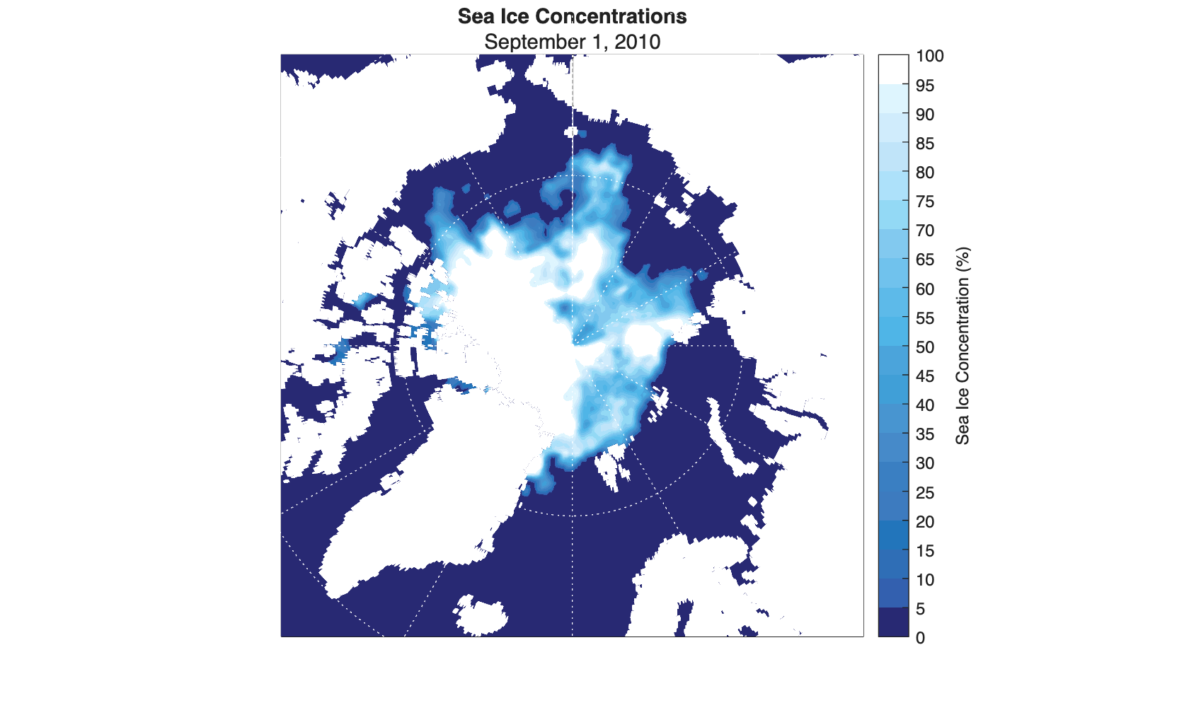
This GRIB file contains multi-year sea ice concentration data from the Copernicus Climate Data Store in ECMWF and stores the data as a grid of posting point samples referenced to geographic coordinates.[1][2]
Get Information About the GRIB File
The first command we'll look at is georasterinfo which we'll use to create a RasterInfo object that puts all of the GRIB metadata into a table, where each row of the table corresponds to a band of data in the file.
In this file, each data band corresponds to a year. The meaning of bands in GRIB is file-specific; here bands correspond to years, but in other files they may correspond to a different variable.
info = georasterinfo("seaice.grib");
info.Metadata
Read Data Band
Using the readgeoraster command, we read the data band for 2010, which corresponds to the first row in the metadata table and hence the first band. Then, convert the concentrations to percentages.
[iceConcentration2010,R2010] = readgeoraster("seaice.grib",Bands=1);
percentIce2010 = 100*iceConcentration2010;
Get the reference time for the band.
refTime2010 = info.Metadata.ReferenceTime(1);
refTime2010 = string(refTime2010,"MMMM d, yyyy");
Display Data Band
Load an ice colormap that is appropriate for ice concentration data. The colormap starts at dark blue and transitions to light blue and white.
load iceColormap.mat
Specify ice concentration levels from 0% to 100%. The level increases every 5%.
levels = 0:5:100;
Set up an axesm-based map for an arctic region using a polar stereographic projection.
figure
abm = axesm("stereo",Origin=[90 0 0],Grid="on",GColor="w");
Zoom into the arctic region.
nlim = 0.45;
set(abm,XLim=[-nlim nlim],YLim=[-nlim nlim])
Set colormap and color limits.
colormap(iceColormap)
clim(abm,[min(levels) max(levels)])
Add a labeled color bar.
cb = colorbar;
cb.Ticks = levels;
cb.Label.String = "Sea Ice Concentration (%)";
Provide geographic context for the map by displaying world land areas in gray. Then, display the sea ice concentrations as a surface. To make the surface appear under the land areas, display a matrix of zeros and apply color using the ice concentrations.
land = readgeotable("landareas.shp");
landColor = [0.8 0.8 0.8];
geoshow(land,FaceColor=landColor)
geoshow(zeros(R2010.RasterSize),R2010,DisplayType="surface",CData=percentIce2010)
Add a title and subtitle.
title("Sea Ice Concentrations")
subtitle(refTime2010)
This example is a shortened version of the documentation example Visualize Sea Ice Concentrations from GRIB Data which also shows how to create an animation that depicts the variations in sea ice concentration over time.
References
[1] Hersbach, H., B. Bell, P. Berrisford, G. Biavati, A. Horányi, J. Muñoz Sabater, J. Nicolas, et al. "ERA5 Hourly Data on Single Levels from 1940 to Present." Copernicus Climate Change Service (C3S) Climate Data Store (CDS), 2023. Accessed May 22, 2023. https://doi.org/10.24381/cds.adbb2d47.
[2] Neither the European Commission nor ECMWF is responsible for any use that may be made of the Copernicus information or data it contains.
- Category:
- geoscience,
- Mapping,
- New Features


Comments
To leave a comment, please click here to sign in to your MathWorks Account or create a new one.