
A look at some of what’s new in MATLAB R2026b
My various social media feeds are full of discussion of the September "Back-to-school" reset. I feel it too, even though it's now 30 years since I started my undergraduate physics degree at The University of Sheffield. I have the urge to declutter, buy new stationery and, of course, update my MATLAB!
R2026b was released on 23rd September 2026 and contains some features that we've been working on for a long time. As always, I urge you to dig into the detailed release notes to see everything that we've built for you. For now, I hope you enjoy this tour of my favorite new features across the MATLAB Ecosystem.
MATLAB Package Management
You can now install community packages from File Exchange using mpminstall. For example, let's install FSDA (Flexible Statistics Data Analysis) toolbox.
mpminstall fsda
You will be accessing content made available under separate license terms.
License terms are available in the package installation folder.
The following packages will be installed:
fsda@8.7.11 (Repository: File Exchange Repository)
Do you want to continue? [YES/no]:
Press Enter to accept the default (YES) and you're done
Successfully installed the following packages:
fsda@8.7.11 (help)
Installation complete.
You can list all installed packages with mpmlist
mpmlist
mpmuninstall fsda
The following packages will be uninstalled:
fsda@8.7.11
Do you want to continue? [YES/no]:
Uninstallation complete.
There is a lot more to dig into here including things like dependencies between packages, alternative repositories and the best way to create them. There will be follow-up posts about this new workflow on The MATLAB Blog soon.
The enhanced command window
Functions such as fprintf now render ANSI escape codes in the command window which allows you to output styled and colored text in the command window. For example:

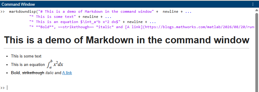
The new markdowndisp function allows you to render markdown text in the command window using GitHub Flavored Markdown.
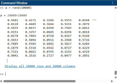
Finally, the Command Window now truncates most large two‑dimensional numeric matrices by default.
Expect a more in-depth article on these new Command Window features soon.
Plain text file formats for App Designer apps and Live Scripts
In previous versions of MATLAB, App Designer apps have only been able to use the .mlapp binary format which is not very source-control friendly. As of R2026b, you can now choose to save apps in a plain text format which is a combination of .m and .xml files. The default is currently still .mlapp but I encourage you to try out the new file format. More details can be found in this blog post by one of our developers: Plain-Text MATLAB Apps in R2026b: A Diff You Can Read
Live scripts went through a similar transition last year. Originally, only the binary .mlx file format was available but R2025a introduced the plain text .m Live Code Format as an option. In R2026b, this plain text format is now the default for live scripts with the .mlx format becoming the option.
Google Sheets support
MATLAB now includes full Google Sheets support. Once you've connected MATLAB to your Google account, all of the standard functions such as readtable, writetable, readmatrix, writematrix, readcell, writecell, readtimetable, writetimetable, and sheetnames will work just as you'd expect them to. For example, to read a Google Sheets spreadsheet, you'd do something like
url = "https://docs.google.com/spreadsheets/d/SPREADSHEET_ID";
T = readtable(url);
Design of Experiments (DOE)
Over the last few releases, an object oriented framework for Design of Experiments has been built out in Statistics and Machine Learning Toolbox. This continues in R2026b with the new responseSurfaceDOE object and the new addReplicates and randomizeRunOrder functions which round out a comprehensive new framework that first appeared in R2024b.
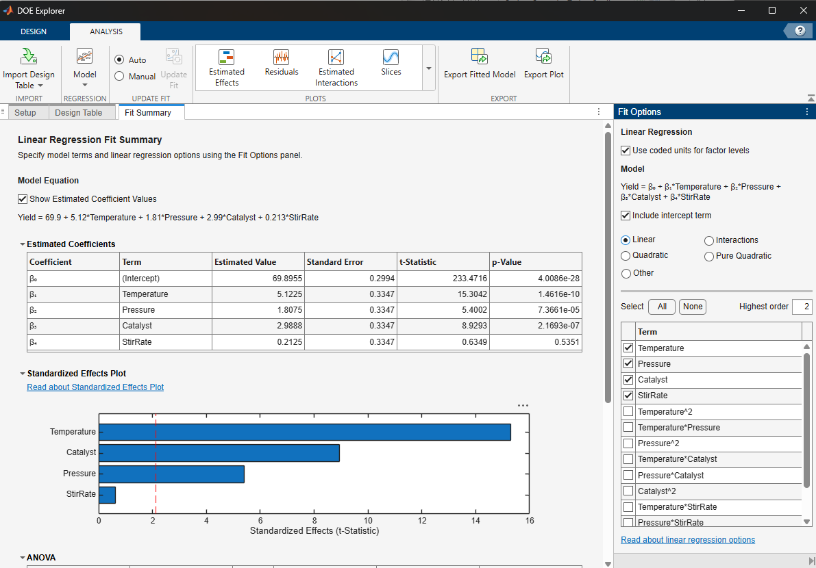
In addition to this programmatic framework, R2026b sees the release of the DOE Explorer App which exposes the entire workflow in a graphical user interface. For more details on the app, refer to this 4 minute video.
Pass GPU data between MATLAB and Python
Once you've got your data in GPU memory, you usually want to keep it there for as long as possible since data transfers to and from host memory can kill performance. These new features in Parallel Computing Toolbox and Deep Learning Toolbox allow you to combine MATLAB and Python GPU workflows without a round trip through host memory.
To demonstrate, I first need a version of Python with CuPy, PyTorch and TensorFlow installed. The Python on my machine was pretty out of date so I used the MATLAB Support for Python 3.13 package (also new at R2026b) to update to Python 3.13 just for MATLAB. R2026b also supports Python 3.14 but that's not available as a support package yet. I then used the External Languages Panel (new in R2026a) to select Python 3.13, select 'run Python in a separate process' and install CuPy, PyTorch and TensorFlow.
The set up done, I start by creating a 1 million element random array on the GPU using MATLAB
x = 600* rand(1000,"gpuArray");
pyx = pycupyarray(x);
Let's compute something on the GPU using CuPy
pyw = py.cupyx.scipy.special.wright_bessel(0.01, 0, pyx);
Then transfer the result back to MATLAB
w = gpuArray(pyw);
As you can see, the workflow is straightforward but it's worth noting that the transfer between processes isn't free. After running the four lines above, my GPU contains two copies of the input data, x and pyx, and two copies of the output data, pyw and w. If you are dealing with large arrays, you'll need to pay careful attention to memory management when using this functionality.
CuPy isn't the only Python framework supported on the GPU. We can also inter-operate with PyTorch with arrayToTorchTensor and torchTensorToArray.
B = rand(2,3,4,"gpuArray");
Q = arrayToTorchTensor(B);
Q.size()
GPU Monitor
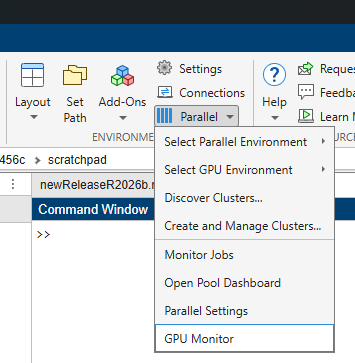
Now that we have additional ways to use our GPU in MATLAB, it's timely that we also have a way to monitor GPU usage via the GPU Monitor App. To launch it, click on Parallel in the Environment Tab and then GPU Monitor.
The app shows GPU Memory Usage and GPU Utilization in real time. I only have one NVIDIA GPU on my machine but if you are lucky enough to have several, multiple GPUs are supported
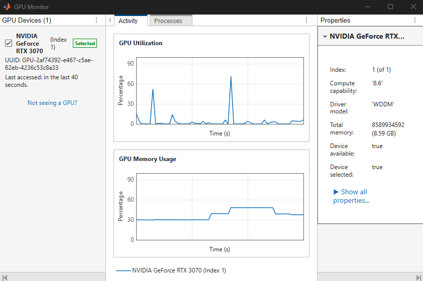
When I took the screenshot above, I had been creating and destroying GPU arrays in MATLAB but I should point out that this isn't just MATLAB's utilization of the GPU. It covers all processes. So, when I later ran a Large Language Model using Ollama, I saw how that affected GPU memory and utilisation as well.
Improved performance in MATLAB R2026b
I wrote about the improvements to the MATLAB object management system earlier this year and showed that some operations have been made over 300x faster! Back then, this new feature was only available via a limited beta and you had to contact MathWorks support to get access to it. In R2026b, you can turn it on by installing the Object Performance Improvement for MATLAB (Beta). As I discussed in my article, this is a fundamental language performance improvement and you will discover that many different workflows will be made faster. If it involves objects, there's a good chance you'll see an improvement although the actual amount of speed-up can vary dramatically depending on how your code uses objects.
Outside of this system-wide improvement, R2026b sees the usual raft of speed optimizations you've come to expect from a new MATLAB release. For the full list, check out the Performance category of the release notes.
Some of my favorites include
- Up to 94x speed-up for union(v) and intersect(v) when v is a vector of polyshape objects.
- Several operations on datetime arrays have been made faster with up to 43x speed-up shown in the release notes.
- Various graphics and desktop speed enhancements such as Improved scrolling on high-DPI displays in MATLAB Editor, improved responsiveness for the plot and plot3 functions and improved performance when resizing an app with multiple sliders in a grid.
- Deep Learning Training: There have been a couple of improvements to trainnet from Deep Learning Toolbox. You can now speed up GPU training using automatic mixed precision which uses half-precision under the hood. CPU training has also been made faster with the example in the release notes showing a 1.7x speed-up.
With some of these very specific speed improvements, it can sometimes be difficult to see why you should care. For example, validatestring has been improved in R2026b with the example in the release note showing a 5.8x speed-up. Your immediate thought might be 'I never use validatestring so I don't care'. However, it turns out that hundreds of functions in base MATLAB and the various toolboxes do use it; usually (but not always) as part of argument handling so all of these will be a little bit faster too.
For many functions, the time taken by validatestring, before and after this update, is often negligible compared to the rest of the work that the function does. This brings us back to 'why should I care?'. However, this update is part of a wider pattern you'll have seen over the last few years: The MATLAB language is consistently getting faster.
Sometimes we make a big deal out of this such as when function handles were made faster in R2023a or the big object optimizations I discussed above. Other times it's just an entry in the release notes. Some improvements are made incidentally and don't even make the release notes at all. One example being my discovery that vector concatenation was made slightly faster in R2024b.
3D Scenarios in Mapping Toolbox
The new 3D Scenarios add-on to Mapping Toolbox enables you to build, visualize, and simulate scenarios in a 3D geographic environment and I created the animation below by working through the Create 3D Scenarios example in R2026b. The simulation is of a car traveling through Manhattan, using real buildings data obtained from OpenStreetMap and a programmatically defined driving route.
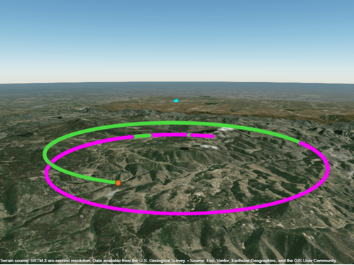
The line that follows the car is a line-of-sight calculation from a simulated tower that's located just above one of the buildings. When it's a dotted red-line, the car cannot be seen from the tower and when it's green, it can.
Another built-in example swaps the car for an aircraft. The Visualize Aircraft Line-of-Sight over Terrain example uses terrain data from the United States Geological Survey (USGS) of an area around Boulder, Colorado in the USA. It defines a radar ground location at Rocky Mountain Metropolitan Airport and simulates a circular flight path. I could have created a similar animation to the one above but I'll just leave you with a visualization of the LOS analysis.
Did I miss your favorite update?
I had hundreds of updates to choose from and I only selected 9. Take a look at the release notes for yourself and pick out your favorites for R2026b. Let me know in the comments.


댓글
댓글을 남기려면 링크 를 클릭하여 MathWorks 계정에 로그인하거나 계정을 새로 만드십시오.