Spatial transformations: Where is the input image?

저자 Steve Eddins, February 28, 2006

1 회 조회 (최근 30일) | 0 좋아요 | 23 댓글

We've talked about using Image Processing Toolbox functions to define an affine transformation and apply it to points. Let's begin to explore transforming images.

First we have to answer a question that is often overlooked: Where is the input image? In other words, the input u-v space is a plane. Where does the image lie on the plane?

Image location in the plane
Rotation
Scaling

Image location in the plane

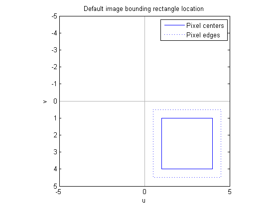
With the default spatial coordinates for images in MATLAB, the center of the upper-left image pixel is at (1, 1). Each pixel is a square with unit area, so the corner of the upper-left image pixel is at (0.5, 0.5). A 4-by-4 image looks like this on the plane:

pixel_centers_x = [1 4 4 1 1];
pixel_centers_y = [1 1 4 4 1];
pixel_edges_x   = [0.5 4.5 4.5 0.5 0.5];
pixel_edges_y   = [0.5 0.5 4.5 4.5 0.5];

plot(pixel_centers_x, pixel_centers_y);
hold on
plot(pixel_edges_x, pixel_edges_y, ':')

% Plot axes lines
c = [.7 .7 .7];
plot([-50 50], [0 0], 'color', c);
plot([0 0], [-50 50], 'color', c);

axis ij, axis equal
axis([-5 5 -5 5]);

legend({'Pixel centers', 'Pixel edges'})
title('Default image bounding rectangle location')
xlabel('u')
ylabel('v')
hold off

Rotation

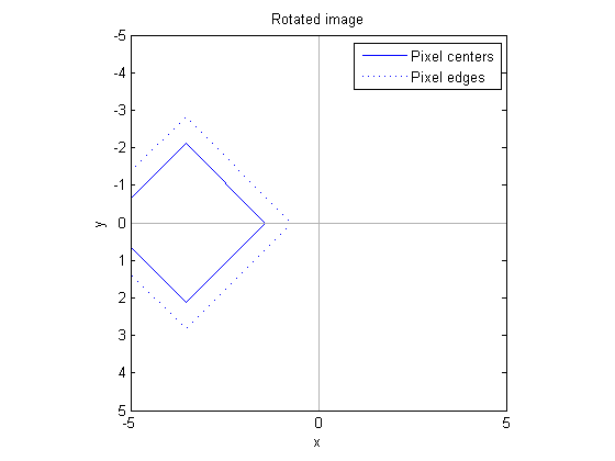
A "pure" affine rotation rotates about the origin. This means it can move an image into a completely different quadrant from where it started.

theta = 3*pi/4;
A1 = [ cos(theta)  sin(theta)  0
      -sin(theta)  cos(theta)  0
       0           0           1];

tform1 = maketform('affine', A1);

[pixel_centers_x1, pixel_centers_y1] = tformfwd(tform1, ...
   pixel_centers_x, pixel_centers_y);
[pixel_edges_x1, pixel_edges_y1] = tformfwd(tform1, ...
   pixel_edges_x, pixel_edges_y);

plot(pixel_centers_x1, pixel_centers_y1);
hold on
plot(pixel_edges_x1, pixel_edges_y1, ':')

% Plot axes lines
c = [.7 .7 .7];
plot([-50 50], [0 0], 'color', c);
plot([0 0], [-50 50], 'color', c);

axis ij, axis equal
axis([-5 5 -5 5]);

legend({'Pixel centers', 'Pixel edges'})
title('Rotated image')
xlabel('x')
ylabel('y')
hold off

Scaling

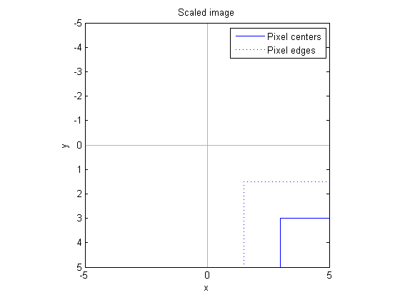
A "pure" affine scaling also operates with respect to the origin. Since the image corner isn't exactly at the origin (by default), scaling with a scale factor greater than 1 not only increases the size of the pixels, but it also moves the corner of the image away from the origin.

A2 = [ 3  0  0
       0  3  0
       0  0  1];

tform2 = maketform('affine', A2);

[pixel_centers_x2, pixel_centers_y2] = tformfwd(tform2, ...
   pixel_centers_x, pixel_centers_y);
[pixel_edges_x2, pixel_edges_y2] = tformfwd(tform2, ...
   pixel_edges_x, pixel_edges_y);

plot(pixel_centers_x2, pixel_centers_y2);
hold on
plot(pixel_edges_x2, pixel_edges_y2, ':')

% Plot axes lines
c = [.7 .7 .7];
plot([-50 50], [0 0], 'color', c);
plot([0 0], [-50 50], 'color', c);

axis ij, axis equal
axis([-5 5 -5 5]);

legend({'Pixel centers', 'Pixel edges'})
title('Scaled image')
xlabel('x')
ylabel('y')
hold off

The center of the upper-left pixel is now at (3, 3), and the corner of the upper-left pixel is now at (1.5, 1.5).

When I discuss imtransform, I'll explain how it automatically takes care of these details so that most users don't have to worry about it. But if you want to understand how things work, or if imtransform's automatic procedure doesn't do exactly what you need, then you need to understand this information.

Published with MATLAB® 7.1