
Spatial transformations: Defining and applying custom transforms
Blog reader David A. asked me a while back about how to transform an image based on some mathematical function. For example, the online paper "Visualizing complex analytic functions using domain coloring," by Hans Lundmark, has an example of defining a spatial transformation by assuming that the input and output spaces are complex planes, and that the inverse mapping is given by:
Check out Figure 3 in the paper to see what this does to an image.
You can use maketform to create a custom spatial transformation by supplying your own function handle to perform the inverse mapping. Your function handle has to take two input arguments. The first input argument is a P-by-ndims matrix of points, one per row. (imtransform applies two-dimensional spatial transformations, so I'll be using P-by-2 matrices here.) The second argument, called tdata, can be used to pass auxiliary information to your function handle. My examples will just ignore this second argument.
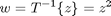
Let's start with a very simple example just to illustrate the mechanics. Make an inverse mapping that just swaps the horizontal and vertical coordinates:
% inverse mapping function
f = @(x, unused) fliplr(x);

% maketform arguments
ndims_in = 2;
ndims_out = 2;
forward_mapping = [];
inverse_mapping = f;
tdata = [];
tform = maketform('custom', ndims_in, ndims_out, ...
    forward_mapping, inverse_mapping, tdata);

body = imread('liftingbody.png');
body2 = imtransform(body, tform);

subplot(1,2,1)
imshow(body)
subplot(1,2,2)
imshow(body2)
As we might have guessed, this custom transform just transposes the image.
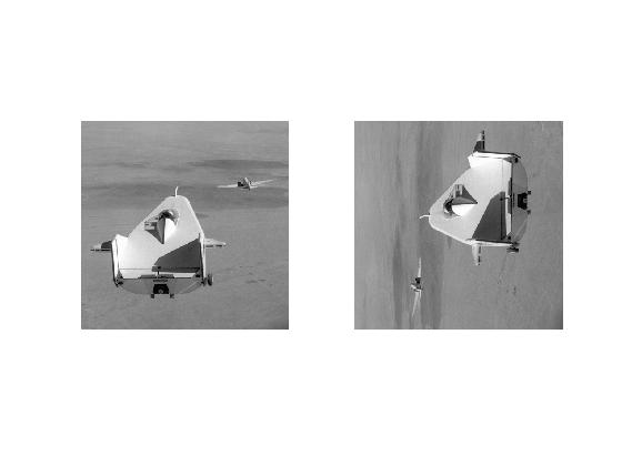
For my other examples I'll use a picture of someone I know well:
face = imread('https://blogs.mathworks.com/images/steve/74/face.jpg');
clf
imshow(face)
There is a fun little book called Beyond Photography: The Digital Darkroom, by Gerard Holzmann. This book has lots examples of spatial transformations based on simple mathematical expressions. Here's one that uses the square root of the polar radial component.
Note that the call to imtransform below sets up the input image to be located in the square from -1 to 1 in both directions. The output image grid is set up to be the same square.
r = @(x) sqrt(x(:,1).^2 + x(:,2).^2);
w = @(x) atan2(x(:,2), x(:,1));
f = @(x) [sqrt(r(x)) .* cos(w(x)), sqrt(r(x)) .* sin(w(x))];
g = @(x, unused) f(x);

tform2 = maketform('custom', 2, 2, [], g, []);
face2 = imtransform(face, tform2, 'UData', [-1 1], 'VData', [-1 1], ...
    'XData', [-1 1], 'YData', [-1 1]);
imshow(face2)

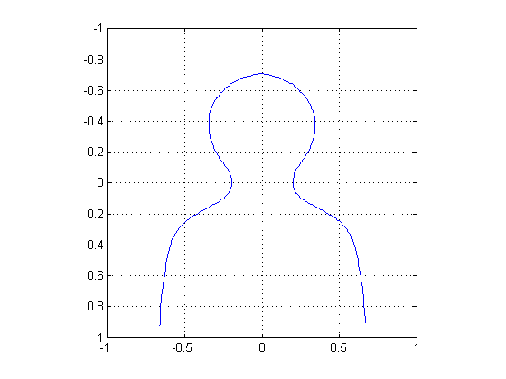
This example uses the square of polar radial component.
f = @(x) [r(x).^2 .* cos(w(x)), r(x).^2 .* sin(w(x))];
g = @(x, unused) f(x);

tform3 = maketform('custom', 2, 2, [], g, []);
face3 = imtransform(face, tform3, 'UData', [-1 1], 'VData', [-1 1], ...
    'XData', [-1 1], 'YData', [-1 1]);
imshow(face3)

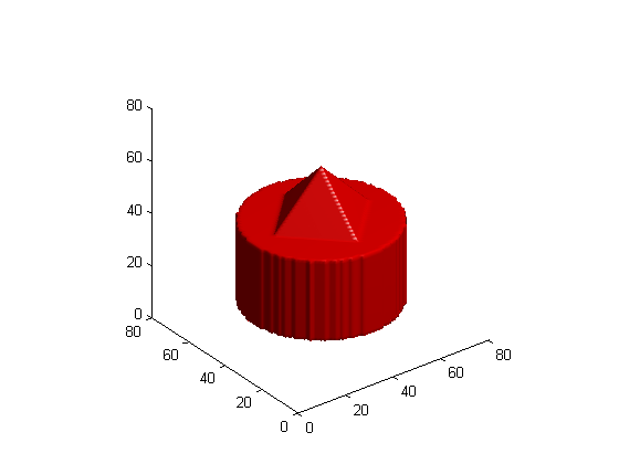
Finally, let's try the complex-plane function used in Lundmark's article. I'll construct the inverse mapping function in several steps: First, convert output-space Cartesian coordinates to complex values; square the complex values; and then produce new input-space Cartesian coordinates from the squared complex values.
f = @(x) complex(x(:,1), x(:,2));
g = @(z) z.^2;
h = @(w) [real(w), imag(w)];
q = @(x, unused) h(g(f(x)));

tform4 = maketform('custom', 2, 2, [], q, []);
face4 = imtransform(face, tform4, 'UData', [-1 1], 'VData', [-1 1], ...
    'XData', [-1 1], 'YData', [-1 1]);
imshow(face4)

If you want see to more examples of this kind of mathematical image fun, take a look at "Exploring a Conformal Mapping" in the Image Processing Toolbox product examples area.
- カテゴリ:
- Spatial transforms


コメント
コメントを残すには、ここ をクリックして MathWorks アカウントにサインインするか新しい MathWorks アカウントを作成します。