Upslope area – D-infinity flow
A few weeks ago I promised a series on developing a MATLAB algorithm to compute upslope area. Now I'm ready to begin that project in earnest.
First, though, I'd like to comment on the motivation for this series. Specifically, why look at a method from the area of hydrology in a blog about image processing algorithms? There are two reasons:
- MATLAB users are in all disciplines of engineering and science, and the ones who use image processing methods use them for a variety of gridded data sets, not just for processing pictures. Applying image processing techniques to digital elevation models (DEMs), for example, is common.
- Several techniques originally developed for the computational analysis of DEMs have turned out to be broadly useful for processing other kinds of image data. Perhaps the most well-known example is the watershed transform.
The first thing we need to think about is computing the flow direction for a given pixel. That is, based on the height of a pixel and its neighbors, in which direction will water run off from the center of that pixel? The Tarboton 1997 paper says the earliest method is to say the flow direction is toward whichever of the eight neigbhors has the steepest downward slope. Because the flow direction can take on one of 8 possible values, this is called the D8 method.
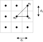
Tarboton proposes a new flow direction method, called D-infinity because flow direction assigned to a pixel can take on any value between 0 and 2*pi. The method examines eight triangular facets for each pixel. Each facet has a vertex at the pixel center and two vertices at the centers of neighboring pixels.

The flow direction for a particular facet is the direction of the steepest downward slope on the facet. The function facetFlow below computes this value for the east-northeast facet. Variable names in the code are based on this diagram:

type facetFlow
function [r,s] = facetFlow(e0, e1, e2, d1, d2)
% facetFlow Facet flow direction.
% [r, s] = facetFlow(e0, e1, e2, d1, d2) computes the facet flow direction
% for an east-northeast pixel facet.  e0 is the height of the center pixel.
% e1 is the height of the east neighbor.  e2 is the height of the northeast
% neighbor.  d1 is the horizontal pixel center spacing.  d2 is the vertical
% pixel center spacing.  d1 and d2 are optional; if omitted, a value of 1.0
% is assumed.
%
% r is the facet flow direction in radians, and s is the magnitude of the
% corresponding slope.

% Steve Eddins
% Copyright 2007 The MathWorks, Inc.

% Reference: Tarboton, "A new method for the determination of flow
% directions and upslope areas in grid digital elevation models," Water
% Resources Research, vol. 33, no. 2, pages 309-319, February 1997.

if nargin < 4
    d1 = 1;
    d2 = 1;
end

s1 = (e0 - e1)/d1;             % eqn (1)
s2 = (e1 - e2)/d2;             % eqn (2)

r = atan2(s2, s1);             % eqn (3)
s = hypot(s1, s2);             % eqn (3)

diagonal_angle    = atan2(d2, d1);
diagonal_distance = hypot(d1, d2);

if r < 0
    % eqn (4)
    r = 0;
    s = s1;

elseif r > diagonal_angle
    % eqn (5)
    r = diagonal_angle;
    s = (e0 - e2)/diagonal_distance;
end
This same computation can be applied to all the facets via rotations or flips. Tarboton provides a lookup table of facet transformations that can be used directly in the implementation. The function pixelFlow below uses facetFlow and the lookup table to find both the flow direction and flow magnitude for a given pixel inside a DEM matrix. The flow direction for the pixel is the flow direction with the highest magnitude for each of the eight facets.
type pixelFlow
function [r, s] = pixelFlow(E, i, j, d1, d2)
% pixelFlow Downslope flow direction from a pixel in a DEM.
% [r, s] = pixelFlow(E, i, j, d1, d2) computes the flow direction for a
% single DEM pixel E(i, j).  d1 is the horizontal pixel center spacing.  d2
% is the vertical pixel center spacing.  d1 and d2 are optional; if
% omitted, a value of 1.0 is assumed.
%
% r is the facet flow direction in radians, and s is the magnitude of the
% corresponding slope.

% Steve Eddins
% Copyright 2007 The MathWorks, Inc.

% Reference: Tarboton, "A new method for the determination of flow
% directions and upslope areas in grid digital elevation models," Water
% Resources Research, vol. 33, no. 2, pages 309-319, February 1997.

if nargin < 4
    d1 = 1;
    d2 = 1;
end

% Table 1, page 311
e0 = E(i, j);
e1 = [E(i,j+1) E(i-1,j) E(i-1,j) E(i,j-1) ...
      E(i,j-1) E(i+1,j) E(i+1,j) E(i,j+1)];

e2 = [E(i-1,j+1) E(i-1,j+1) E(i-1,j-1) E(i-1,j-1) ...
      E(i+1,j-1) E(i+1,j-1) E(i+1,j+1) E(i+1,j+1)];

ac = [0  1  1  2  2  3  3  4];
af = [1 -1  1 -1  1 -1  1 -1];

rp = zeros(1, 8);
sp = zeros(1, 8);

for k = 1:8
    [rp(k), sp(k)] = facetFlow(e0, e1(k), e2(k), d1, d2);
end

% Find the facet with the maximum down-slope.
[s, k_max] = max(sp);

if s > 0
    % Maximum down-slope is positive.
    r = (af(k_max) * rp(k_max)) + (ac(k_max) * pi / 2);
else
    % The pixel is in a flat area or is a pit.  Flow direction angle is
    % unresolved.
    r = NaN;
end
Note: At this point in algorithm development, I am primarily concerned with getting a correct implementation of the method described in the paper. It's way too early yet to be worrying about performance. Also, note the cross-references in my code to specific equation and page numbers. This is a really good habit to get into. (I learned that lesson the hard way.)
Next up: Try this pixel flow computation on some simple test cases, and start to think about what to do for plateaus.
- カテゴリ:
- Upslope area


コメント
コメントを残すには、ここ をクリックして MathWorks アカウントにサインインするか新しい MathWorks アカウントを作成します。