Logical indexing
This is the first post in a short series on index techniques that are particularly useful for image processing in MATLAB. I'll start with logical indexing today. Later I'll cover linear indexing, and then a technique I like to call neighbor indexing.
Every MATLAB user is familiar with ordinary matrix indexing notation.
A = magic(5)
A =

    17    24     1     8    15
    23     5     7    14    16
     4     6    13    20    22
    10    12    19    21     3
    11    18    25     2     9
A(2,3)
ans =

     7
A(2,3) extracts the 2nd row, 3rd column of the matrix A. You can extract more than one row and column at the same time:
A(2:4, 3:5)
ans =

     7    14    16
    13    20    22
    19    21     3
When an indexing expression appears on the left-hand side of the equals sign, it's assignment:
A(5,5) = 100
A =

    17    24     1     8    15
    23     5     7    14    16
     4     6    13    20    22
    10    12    19    21     3
    11    18    25     2   100
About every 13.6 days, someone asks this question on comp.soft-sys.matlab:
How do I replace all the NaNs in my matrix B with 0s?
This is generally followed 4.8 minutes later with this reply from one of the newsgroup regulars:
B(isnan(B)) = 0;
For example:
B = rand(3,3);
B(2, 2:3) = NaN
B =

    0.5470    0.1890    0.3685
    0.2963       NaN       NaN
    0.7447    0.1835    0.7802
Replace the NaNs with zeros:
B(isnan(B)) = 0
B =

    0.5470    0.1890    0.3685
    0.2963         0         0
    0.7447    0.1835    0.7802
The expression
B(isnan(B))
is an example of logical indexing. Logical indexing is a compact and expressive notation that's very useful for many image processing operations.
Let's talk about the basic rules of logical indexing, and then we'll reexamine the expression B(isnan(B)).
If C and D are matrices, then C(D) is a logical indexing expression if C and D are the same size, and D is a logical matrix.
"Logical" is one of the builtin types, or classes, of MATLAB matrices. Relational operators, such as == or >, produce logical matrices.
C = hilb(4)
C =

    1.0000    0.5000    0.3333    0.2500
    0.5000    0.3333    0.2500    0.2000
    0.3333    0.2500    0.2000    0.1667
    0.2500    0.2000    0.1667    0.1429
D = C > 0.4
D =

     1     1     0     0
     1     0     0     0
     0     0     0     0
     0     0     0     0
whos DName Size Bytes Class Attributes D 4x4 16 logical
You can see from the output of whos that the class of the variable D is logical. The logical indexing expression C(D) extracts all the values of C corresponding to nonzero values of D and returns them as a column vector.
C(D)
ans =

    1.0000
    0.5000
    0.5000
Now we know enough to break down the B(isnan(B)) example to see how it works.
B = rand(3,3);
B(2, 2:3) = NaN;

nan_locations = isnan(B)
nan_locations =

     0     0     0
     0     1     1
     0     0     0
whos nan_locationsName Size Bytes Class Attributes nan_locations 3x3 9 logical
B(nan_locations)
ans =

   NaN
   NaN
B(nan_locations) = 0
B =

    0.0811    0.4868    0.3063
    0.9294         0         0
    0.7757    0.4468    0.5108
Functions in the Image Processing Toolbox, as well as the MATLAB functions imread and imwrite, follow the convention that logical matrices are treated as binary (black and white) images. For example, when you read a 1-bit image file using imread, it returns a logical matrix:
bw = imread('text.png');
whos bw
  Name        Size             Bytes  Class      Attributes

  bw        256x256            65536  logical
This convention, together with logical indexing, makes it very convenient and expressive to use binary images as pixel masks for extracting or operating on sets of pixels.
Here's an example showing how to use logical indexing to compute the histogram of a subset of image pixels. Specifically, given a gray-scale image and a binary segmentation, compute the histogram of just the foreground pixels in the image.
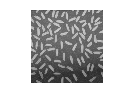
Here's our original image:
I = imread('rice.png');
imshow(I)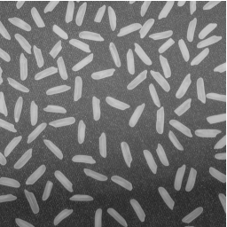
Here's a segmentation result (computed and saved earlier), represented as a binary image:
url = 'https://blogs.mathworks.com/images/steve/192/rice_bw.png';
bw = imread(url);
imshow(bw)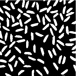
Now use the segmentation result as a logical index into the original image to extract the foreground pixel values.
foreground_pixels = I(bw);
whos foreground_pixels
Name Size Bytes Class Attributes foreground_pixels 17597x1 17597 uint8
Finally, compute the histogram of the foreground pixels.
imhist(foreground_pixels)
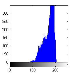
Or use logical indexing with the complement of the segmentation result to compute the histogram of the background pixels.
imhist(I(~bw))
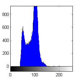
- カテゴリ:
- Indexing




コメント
コメントを残すには、ここ をクリックして MathWorks アカウントにサインインするか新しい MathWorks アカウントを作成します。