Neighbor indexing
Earlier this year I wrote about logical indexing and linear indexing.
Now I want to finish this little indexing series with an example of a technique I call neighbor indexing. I've written about neighbor indexing before, but in this post I'll show a more complete example of its application to image processing.
Many image processing operations can be classified as recursive neighborhood operations. (Thanks to Chris for suggesting this term to me.) You do something to each neighbor of a pixel, then you do something to each neighbor of those neighbors, and so on. Flood filling is a good example, and neighbor indexing is a good way to implement this type of operation in MATLAB. If you implement your own image processing algorithms in MATLAB, you'll probably find neighbor indexing useful.
I'll start by reviewing the basics of neighbor indexing, and then I'll show how to use it to implement flood filling.
Let's make a sample 5-by-5 matrix and consider three seed locations, or starting locations.
A = magic(5)
A =

    17    24     1     8    15
    23     5     7    14    16
     4     6    13    20    22
    10    12    19    21     3
    11    18    25     2     9
Starting locations at (2,2), (1,4), (3,4):
rows = [2 1 3];
cols = [2 4 4];
As you'll see, the neighbor indexing technique is based on linear indexing, so let's convert the starting locations to linear indices:
idx = sub2ind(size(A), rows, cols)
idx =

     7    16    18
The linear indices can be used to extract the pixel values of each of the three seed locations:
A(idx)
ans =

     5     8    20
How do you find the linear indices of the eastern neighbor of each of the starting locations?
Answer: Add the number of rows
M = size(A, 1);
east_neighbors = idx + M
east_neighbors =

    12    21    23
M is called the linear offset for the eastern direction.
A(east_neighbors) gives you the pixel values of the eastern neighbors:
A(east_neighbors)
ans =

     7    15    22
What is the linear offset for the northern direction?
northern_offset = -1;
northern_neighbors = idx + northern_offset
northern_neighbors =

     6    15    17
OOPS! The (1,4) pixel doesn't have a northern neighbor! Subtracting 1 from the linear indexing of a pixel on the top row will just give you the pixel on the bottom row of the previous column.
The neighbor indexing technique DOES NOT WORK FOR PIXELS ON THE BORDERS!
Therefore some form of padding is usually necessary.
Here are the offsets corresponding to all eight neighbor directions:
 East         M
 Southeast    M + 1
 South        1
 Southwest   -M + 1
 West        -M
 Northwest   -M - 1
 North       -1
 Northeast    M - 1
The function bsxfun gives you a way to compute all the neighbors of a set of pixels in a single, vectorized expression.
For example, suppose the linear indices of our seed pixels are:
idx = [275 2348 8100]
idx =

         275        2348        8100
And we are interested in finding the north, east, south, and west neighbors of all these pixels:
% Assume a 100-by-100 image for this example.
M = 100;
neighbor_offsets = [-1, M, 1, -M]';
Add every neighbor_offset to every linear index:
neighbors = bsxfun(@plus, idx, neighbor_offsets)
neighbors =

         274        2347        8099
         375        2448        8200
         276        2349        8101
         175        2248        8000
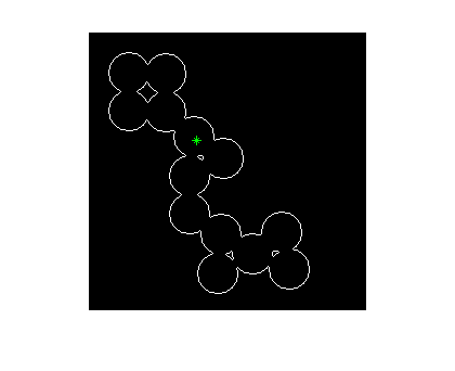
Now we have enough indexing tools to implement a flood-fill algorithm. Let's try it with this image and starting location:
bw = bwperim(imread('circles.png'));
imshow(bw)

r = 100;
c = 100;
hold on
plot(c, r, 'g*')
hold off

Pad the image with ones. This step will prevent the flood filling operation from reaching the border of the image.
bw = padarray(bw, [1 1], 1);
Initialize a linear index array containing the "active pixels." This is the set of pixels to be changed from black to white. Remember that we have to add 1 to the original row and column coordinates because of the padding step above.
active_pixels = sub2ind(size(bw), r+1, c+1);
bw_out = bw;
M = size(bw, 1);
neighbor_offsets = [-1, M, 1, -M];
Our main processing loop will iterate until there are no more active pixels. In each loop iteration, we set the active pixels to 1 in the output image. Then we get all the neighbors of all the active pixels, and we make those neighbors the new active pixels.
That's the basic logic, but there are two special steps you should keep in mind if you use this technique yourself. First, we need to remove from the active pixel list the pixels that are already 1. If we don't do this, the flood fill operation will not stop at the white boundaries.
Second, we need to "dedup" the active pixel list at each iteration. That is, when you find all the neighbors of all the active pixels, there will be duplicates in the list. If you don't prune out the duplicates at each iteration, the number of duplicates can quickly grow to be quite large, causing the algorithm to run slowly and to use a lot of memory.
Here's the main processing loop:
while ~isempty(active_pixels)
    % Set the active pixels to 1.
    bw_out(active_pixels) = 1;

    % The new active pixels list is the set of neighbors of the
    % current list.
    active_pixels = bsxfun(@plus, active_pixels, neighbor_offsets);
    active_pixels = active_pixels(:);

    % Remove from the active_pixels list pixels that are already
    % 1.  This is how we keep the flood fill operation "inside"
    % the white boundaries.
    active_pixels(bw_out(active_pixels)) = [];

    % Remove duplicates from the list.
    active_pixels = unique(active_pixels);
end
Remember to remove the extra padding:
bw_out = bw_out(2:end-1, 2:end-1);
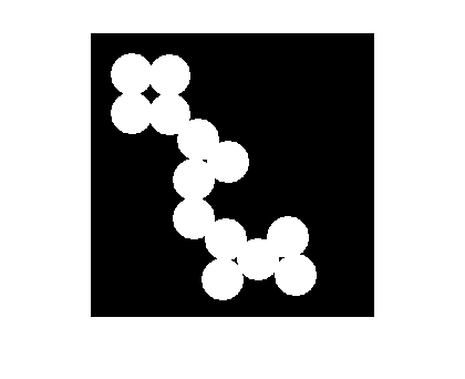
And here's the final result:
imshow(bw_out)

- 범주:
- Indexing


댓글
댓글을 남기려면 링크 를 클릭하여 MathWorks 계정에 로그인하거나 계정을 새로 만드십시오.