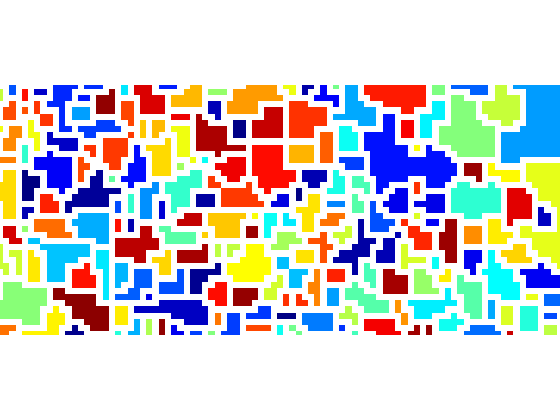
In the previous post in this series on computing the US continental divide, we used the watershed function to find catchment basins in a DEM (digital elevation model). The result was more than half a million catchment basins, most of which were tiny and looked something like this:

Why so many?

To answer this question, let's look at a different kinds of minima in image processing. A local minimum is usually defined as a pixel that is less than or equal to all its neighbors. In a one-dimensional example:

a = [3 2 1 1 1 2 3 4 3 5 6]

a =

     3     2     1     1     1     2     3     4     3     5     6

the third, fourth, fifth, and nineth elements are local minima. A convenient way to find local minima is to use morphological erosion:

imerode(a, [1 1 1]) == a

ans =

     0     0     1     1     1     0     0     0     1     0     0

Now find the local minima in this example:

b = [2 1 1 2 3 4 4 4 5 6]

b =

     2     1     1     2     3     4     4     4     5     6

imerode(b, [1 1 1]) == b

ans =

     0     1     1     0     0     0     1     1     0     0

Now, if you are thinking about the watershed transform and identifying catchment basins, I think you'll agree there's an important distinction between the two groups of local minima (the 1-valued elements and the 4-valued elements) found in b. Water would not accumulate on the flat spot, or plateau, represented by the 4-valued elements; it would instead flow downhill to the left.

That thought leads us to the definition of a regional minimum: a connected group of pixels from which you cannot travel further downhill without going uphill first. The 1-valued elements in b form a regional minima, but the 4-valued elements in b do not.

The Image Processing Toolbox function imregionalmin locates regional minima for you:

imregionalmin(b)

ans =

     0     1     1     0     0     0     0     0     0     0

Let's connect that back to the watershed transform. Every regional minimum is a collection point for water flowing downhill. Thus, there's a one-to-one correspondence between regional minima and catchment basins found by the watershed transform.

Here are all the regional minima pixels in the zoomed-in portion of the DEM that we looked at previously.

% The file continental_divide.mat was created in an earlier post.
s = load('continental_divide');
dem = s.dem_cropped;
reg_min = imregionalmin(dem);
imshow(reg_min, 'InitialMagnification', 'fit');
axis([5580 5670 2060 2100])

We can count the number of regional minima by doing connected-component labeling on the output of imregionalmin.

reg_min_labeled = bwlabel(reg_min);
max(reg_min_labeled(:))

ans =

      540976

That's the same as the number of catchment basins we found in the previous post.

We're on our way to computing just two catchment basins, one for the Pacific Ocean and one for the Atlantic Ocean. Next time we'll take a closer look at the ocean pixels in this data set.

About this Series

This series explores the problem of computing the location of the continental divide for the United States. The divide separates the Atlantic and Pacific Ocean catchment basins for the North American continent.

As an algorithm development problem, computing the divide lets us explore aspects of data import and visualization, manipulating binary image masks, label matrices, regional minima, and the watershed transform.

Data credit: GLOBE Task Team and others (Hastings, David A., Paula K. Dunbar, Gerald M. Elphingstone, Mark Bootz, Hiroshi Murakami, Hiroshi Maruyama, Hiroshi Masaharu, Peter Holland, John Payne, Nevin A. Bryant, Thomas L. Logan, J.-P. Muller, Gunter Schreier, and John S. MacDonald), eds., 1999. The Global Land One-kilometer Base Elevation (GLOBE) Digital Elevation Model, Version 1.0. National Oceanic and Atmospheric Administration, National Geophysical Data Center, 325 Broadway, Boulder, Colorado 80305-3328, U.S.A. Digital data base on the World Wide Web (URL: http://www.ngdc.noaa.gov/mgg/topo/globe.html) and CD-ROMs.

Get the MATLAB code

Published with MATLAB® 7.8