Locating the US continental divide, part 7 – Putting it all together

저자 Steve Eddins, June 5, 2009

1 회 조회 (최근 30일) | 0 좋아요 | 0 댓글

Today is the final post in my continental divide series. In earlier posts I have used the problem of computing the US continental divide as a vehicle for exploring data import, image display scaling, the watershed transform, label matrices, local and regional minima, binary image manipulation, boundary tracing, and visualization techniques.

For this last post, I thought it would useful to gather together all the computational steps in one short script, starting with data import and finishing with the visualization.

% Import the tiles e10g and f10g.
data_size = [6000 10800 1];  % The data has 1 band.
precision = 'int16=>int16';  % Read 16-bit signed ints into a int16 array.
header_bytes = 0;
interleave = 'bsq';          % Band sequential. Not critical for 1 band.
byte_order = 'ieee-le';
E = multibandread('e10g', data_size, precision, header_bytes, ...
    interleave, byte_order);
F = multibandread('f10g', data_size, precision, header_bytes, ...
    interleave, byte_order);
EF = [E, F];

% Crop the data.
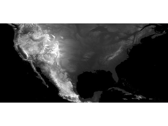
dem = EF(1:4000, 6000:14500);

% Form an ocean mask.
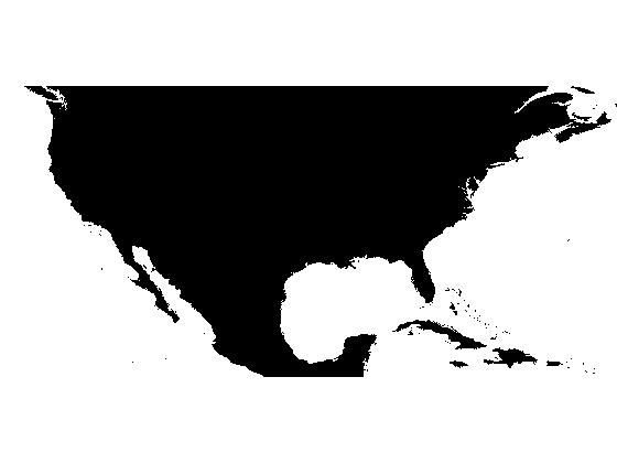
ocean_mask = dem == -500;

% Modify the ocean mask so it contains only the two connected components on
% the left and right side.
[M, N] = size(dem);
ocean_mask = bwselect(ocean_mask, [1 N], [1 1]);

% Modify the DEM so that its only regional minima are the ocean_mask
% pixels.
dem_modified = imimposemin(dem, ocean_mask);

% Compute the watershed transform of the modified DEM.
L = watershed(dem_modified);

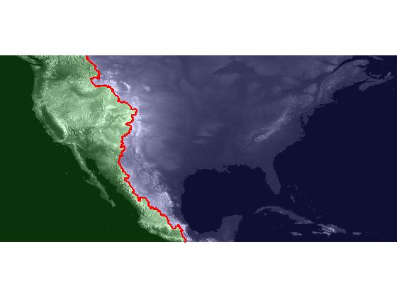
% Visualize the result. First, convert the output of watershed to a color
% image.
pacific = [0.2 1 0.2];
atlantic = [0.3 0.3 1];
ridge = [1 0 0];
rgb = label2rgb(L, [pacific; atlantic], ridge);

% Superimpose the colored watershed image over the DEM.
imshow(dem, [-500 3000], 'InitialMagnification', 'fit')
hold on
h = imshow(rgb);
set(h, 'AlphaData', 0.2);

% Trace the watershed ridge line and superimpose it as a thick red line.
b = bwboundaries(L == 0, 4);
b1 = b{1};  % There's only 1 boundary found here - the ridge line.
x = b1(:,2);
y = b1(:,1);
plot(x, y, 'r', 'LineWidth', 2);

That's it! I hope you enjoyed this series.

Do you have your own ideas for fun computation and visualization using DEM data? Please comment.

About this Series

This series explores the problem of computing the location of the continental divide for the United States. The divide separates the Atlantic and Pacific Ocean catchment basins for the North American continent.

As an algorithm development problem, computing the divide lets us explore aspects of data import and visualization, manipulating binary image masks, label matrices, regional minima, and the watershed transform.

Part 1 - Introduction. Data import and display. multibandread, imshow.

Part 2 - Watershed transform. watershed, label2rgb.

Part 3 - Regional minima. imerode, imregionalmin.

Part 4 - Ocean masks. binary image manipulation, bwselect.

Part 5 - Minima imposition. imimposemin.

Part 6 - Computing and visualizing the divide. watershed, label2rgb, bwboundaries.

Part 7 - Putting it all together. One script that does everything, from data import through computation and visualization of the divide.

Data credit: GLOBE Task Team and others (Hastings, David A., Paula K. Dunbar, Gerald M. Elphingstone, Mark Bootz, Hiroshi Murakami, Hiroshi Maruyama, Hiroshi Masaharu, Peter Holland, John Payne, Nevin A. Bryant, Thomas L. Logan, J.-P. Muller, Gunter Schreier, and John S. MacDonald), eds., 1999. The Global Land One-kilometer Base Elevation (GLOBE) Digital Elevation Model, Version 1.0. National Oceanic and Atmospheric Administration, National Geophysical Data Center, 325 Broadway, Boulder, Colorado 80305-3328, U.S.A. Digital data base on the World Wide Web (URL: http://www.ngdc.noaa.gov/mgg/topo/globe.html) and CD-ROMs.

Published with MATLAB® 7.8