Today, in part 5 of my series on computing the US continental divide, we'll look at a technique called minima imposition. Previously we looked at data import and display, the watershed transform and label matrices, different kinds of minima, and manipulating binary images to form an ocean mask.

In part 3, we found that our DEM data set for the continental US contained more than half a million regional minima, each of which was turned into a catchment basin by the watershed transform. We need a way to get just two catchment basins.

Minima imposition is technique that modifies surface heights, pushing some height values upward so that the resulting surface has regional minima only at specified locations. Minima imposition performs this modification while preserving the local height ordering relationships between neighboring pixels.

Here's a one-dimensional example to illustrate.

a = [1 2 3 4 3 4 3 2 1]

a =

     1     2     3     4     3     4     3     2     1

The vector a has three different regional minima locations:

imregionalmin(a)

ans =

     1     0     0     0     1     0     0     0     1

Let's make a mask representing just two locations where we want to have regional minima:

mask = [1 0 0 0 0 0 0 0 1]

mask =

     1     0     0     0     0     0     0     0     1

This mask says we only want regional minima at each end of the vector, so we want the regional minima in the middle to go away somehow. We do this using the Image Processing Toolbox function imimposemin.

imimposemin(a, mask)

ans =

      -Inf    2.0030    3.0030    4.0030    4.0030    4.0030    3.0030    2.0030      -Inf

The new result has regional minima only at the desired locations. The local minima in the middle of the vector has been pushed up to the level of the surround elements. (As I write this, I am noticing that the small fractional bump that imimposemin gives to all the middle elements seems possibly unnecessary. This is something I will investigate at another time.)

In my previous post I created a binary image representing an ocean mask:

s = load('continental_divide');
dem = s.dem_cropped;
ocean_mask = s.ocean_mask;
imshow(ocean_mask, 'InitialMagnification', 'fit')

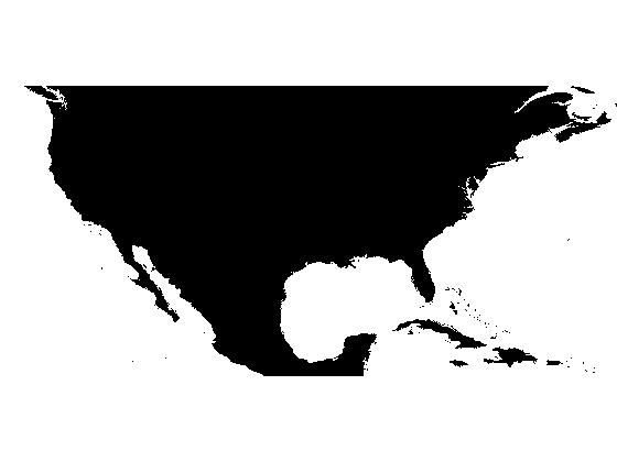
I can use imimposemin, together with the ocean_mask image, to modify the DEM so that the two oceans are the only regional minima.

dem_modified = imimposemin(dem, ocean_mask);

It doesn't look much different:

imshow(dem_modified, [-500 3000], 'InitialMagnification', 'fit')

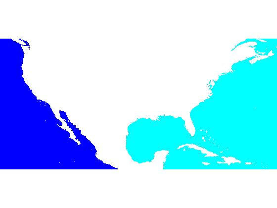
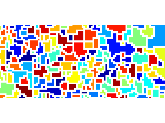
But we can verify that now there are only two regional minima:

regional_minima_labeled = bwlabel(imregionalmin(dem_modified));
max(regional_minima_labeled(:))

ans =

     2

imshow(label2rgb(regional_minima_labeled), 'InitialMagnification', 'fit')

I'll add the modified DEM to the data I've been collecting in continental_divide.mat:

save continental_divide dem_modified -append

Next time I'll perform the final step in computing the continental divide and show one way to visualize it using transparency.

About this Series

This series explores the problem of computing the location of the continental divide for the United States. The divide separates the Atlantic and Pacific Ocean catchment basins for the North American continent.

As an algorithm development problem, computing the divide lets us explore aspects of data import and visualization, manipulating binary image masks, label matrices, regional minima, and the watershed transform.

Data credit: GLOBE Task Team and others (Hastings, David A., Paula K. Dunbar, Gerald M. Elphingstone, Mark Bootz, Hiroshi Murakami, Hiroshi Maruyama, Hiroshi Masaharu, Peter Holland, John Payne, Nevin A. Bryant, Thomas L. Logan, J.-P. Muller, Gunter Schreier, and John S. MacDonald), eds., 1999. The Global Land One-kilometer Base Elevation (GLOBE) Digital Elevation Model, Version 1.0. National Oceanic and Atmospheric Administration, National Geophysical Data Center, 325 Broadway, Boulder, Colorado 80305-3328, U.S.A. Digital data base on the World Wide Web (URL: http://www.ngdc.noaa.gov/mgg/topo/globe.html) and CD-ROMs.

Get the MATLAB code

Published with MATLAB® 7.8