
Fourier transforms, vertical lines, and horizontal lines
A reader asked in a blog comment recently why a vertical line (or edge) shows up in the Fourier transform of an image as a horizontal line. I thought I would try to explain this using the simplest example I could think of.
I'll start with an image that is a constant black except for a single vertical line through the middle of it.
x = zeros(200, 200);
x(:, 100) = 1;
imshow(x)

Next I'll compute and display the log magnitude of the 2-D Fourier transform.
X = fft2(x);
imshow(fftshift(log(abs(X) + 1)), [])

There's the question in black and white, so to speak: Why is there a horizontal line in the 2-D Fourier transform?
Although I'm going to avoid equations and other complicated mumbo-jumbo in my answer, I do have to explain a couple of things about 1-D and 2-D Fourier transforms.
First, the magnitude of the 1-D Fourier transform an "impulse sequence" is a constant. An "impulse sequence" is a sequence that is nonzero only at one place, like this one:
x1 = [0 0 1 0 0]
x1 =

     0     0     1     0     0
The magnitude of the 1-D Fourier transform of x is constant:
abs(fft(x1))
ans =

    1.0000    1.0000    1.0000    1.0000    1.0000
Second, the magnitude of the 1-D Fourier transform of a constant sequence is an impulse. That is, the Fourier transform is nonzero only at one place.
x2 = [1 1 1 1 1]
x2 =

     1     1     1     1     1
abs(fft(x2))
ans =

     5     0     0     0     0
Finally, computing the 2-D Fourier transform is mathematically equivalent to computing the 1-D Fourier transform of all the rows and then computing the 1-D Fourier transforms of all the columns of the result. The order (row-first or column-first) doesn't actually matter.
Now let's go back to x, our 200-by-200 matrix with a vertical line down the middle of it. Each row of x is an impulse sequence:
plot(x(50,:))
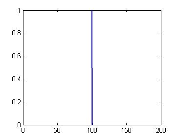
So if we compute the Fourier transform of all the rows, they'll all be constant (in magnitude):
X_rows = fft(x, [], 2);
plot(abs(X_rows(50, :)))
ylim([0 2])

The next step in computing the 2-D Fourier transform is to compute the 1-D Fourier transforms of the columns of X_rows. But those columns are constant. Here's the 100th column of X_rows:
plot(abs(X_rows(:, 100)))
ylim([0 2])
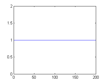
As I said above, the Fourier transform of a constant sequence is an impulse. If you stack up all the resulting columns containing impulse sequences, the result looks like a horizontal line.
X = fft(X_rows, [], 1);
imshow(fftshift(log(abs(X) + 1)), [])

That's a step-by-step computational explanation. Let me leave you with more of a conceptual (that is, hand-wavy) explanation. Let's look at the input image and the 2-D Fourier transform side by side.
subplot(1,2,1)
imshow(x)
title('x')
subplot(1,2,2)
imshow(fftshift(log(abs(X) + 1)), [])
title('Log magnitude of fft2(x)')
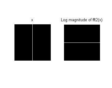
You can think in terms of horizontal and vertical cross-sections. Each horizontal cross-section of x is an impulse sequence. The Fourier transform of an impulse sequence is constant, so horizontal cross-sections of the Fourier transform are constant.
Similarly, each vertical cross-section of x is a constant sequence. The Fourier transform of a constant sequence is an impulse sequence, so the vertical cross-sections of the Fourier transform are impulses. The impulses all line up each other, resulting in the appearance of a horizontal line.
Do these explanations work for you? Do you know of another way to think about it that makes a better explanation? Post your thoughts as comments below.
- カテゴリ:
- Fourier transforms


コメント
コメントを残すには、ここ をクリックして MathWorks アカウントにサインインするか新しい MathWorks アカウントを作成します。