The MATLAB function imwrite writes image data to a variety of different formats including: reads image data from a variety of formats, including JPEG, JPEG 2000, TIFF, PNG, and GIF (as well as a few older formats no longer commonly used).

Probably most people use form where you just provide the image array and a filename.

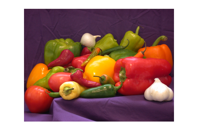
I'll read in one of the sample images in Image Processing Toolbox to experiment with.

rgb = imread('peppers.png');
imshow(rgb)

imwrite(rgb,'mypeppers.tif')

In the above call to imwrite, the function decides which image format to use based on the extension (.tif) in the filename.

Sometimes, though, you might want to use a filename extension for a different purpose. In that case, you call pass a third argument to imwrite to let it know which image format to use.

imwrite(rgb, 'test_image.study_013', 'tif')

Most image file formats support some form of compression. That means that the image takes up less space on disk than you might think based on a simple calculation. For example, the rgb array above takes up about 576 kilobytes in memory.

bytes_in_memory_peppers = numel(rgb)

bytes_in_memory_peppers =

      589824

But it takes less space on disk when you save it to an image format that uses compression. Let's try writing to a PNG file:

imwrite(rgb,'mypeppers.png')

info = imfinfo('mypeppers.png');
bytes_on_disk_peppers_png = info.FileSize

bytes_on_disk_peppers_png =

      287589

compression_ratio = bytes_in_memory_peppers / bytes_on_disk_peppers_png

compression_ratio =

    2.0509

The PNG format uses lossless compression. This means that you can recover the original image data exactly.

peppers2 = imread('mypeppers.png');
isequal(rgb, peppers2)

ans =

     1

Lossless compression methods save a lot more space when the image has large constant areas or contains certain kinds of repetitive, predictable patterns. For example, this image is a screen shot of a MATLAB plot:

url = 'https://blogs.mathworks.com/images/steve/2012/plot_screen_shot.png';
rgb_plot = imread(url);
bytes_in_memory_plot = numel(rgb_plot)

bytes_in_memory_plot =

      336000

info = imfinfo(url);
bytes_on_disk_plot = info.FileSize

bytes_on_disk_plot =

        3284

compression_ratio = bytes_in_memory_plot / bytes_on_disk_plot

compression_ratio =

  102.3143

That's a pretty big compression ratio!

Other image file formats, such as JPEG, use lossy compression. (There is a lossless form of JPEG, but it is obscure and rarely used.) With lossy compression, properties of the human visual system are exploited to reduce the disk size even further, but at a cost --- the original pixels are not exactly recoverable. Let's write out the peppers image using JPEG compression.

imwrite(rgb,'peppers.jpg');
info = imfinfo('peppers.jpg');
bytes_on_disk_peppers_jpg = info.FileSize

bytes_on_disk_peppers_jpg =

       23509

compression_ratio_peppers_jpg = bytes_in_memory_peppers / ...
    bytes_on_disk_peppers_jpg

compression_ratio_peppers_jpg =

   25.0893

That's a much bigger compression ratio than we got with the PNG format above. The cost is in reduced image quality. JPEG does a pretty good job of reducing space without adversely affecting image quality:

imshow('peppers.jpg')

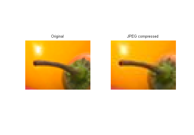
But it isn't perfect, as you can see by zooming in.

subplot(1,2,1)
imshow('peppers.png')
limits = [232 276 215 248];
axis(limits)
title('Original')

subplot(1,2,2)
imshow('peppers.jpg')
axis(limits)
title('JPEG compressed')

You can see the compression artifacts around the stem.

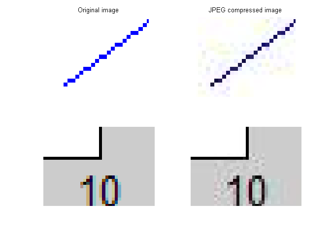
Compression artifacts tend to be more visible on images such as the plot screen shot above.

imwrite(rgb_plot,'plot_screen_shot.jpg')
rgb_plot_compressed = imread('plot_screen_shot.jpg');

subplot(2,2,1)
imshow(rgb_plot)
title('Original image')
limits = [80 105 210 230];
axis(limits);

subplot(2,2,2)
imshow(rgb_plot_compressed)
title('JPEG compressed image')
axis(limits);

subplot(2,2,3)
imshow(rgb_plot)
limits = [345 380 240 265];
axis(limits);

subplot(2,2,4)
imshow(rgb_plot_compressed)
axis(limits);

That's why I usually use PNG for screen shots of many MATLAB graphics. For more complex images, on the other hand, I usually use JPEG.

For more information, see Section 2.4 of Digital Image Processing Using MATLAB.

See also the reference pages for imwrite, as well as the section Reading and Writing Image Data in the Image Processing Toolbox User's Guide.

Get the MATLAB code

Published with MATLAB® 7.13