This is the fourth and last part of my plan (my evil plan?) to rewrite an Image Processing Toolbox example from 20 years ago using more modern MATLAB language features. I got the idea from Dave Garrison's recent article on writing MATLAB apps.

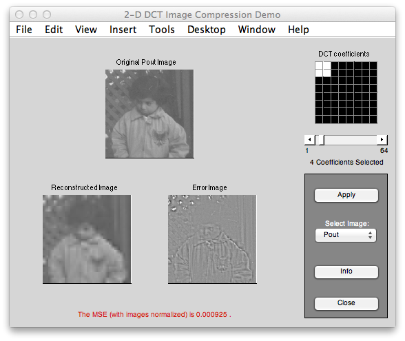
Here's the old app I'm trying to reinvent:

And here's what I had working last time:

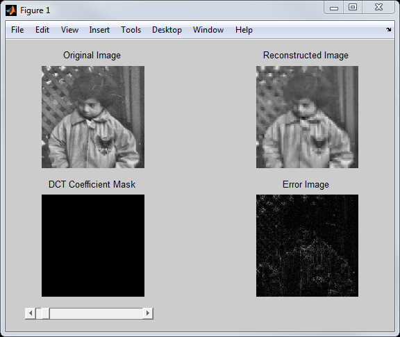
There are two things I want to wrap up before calling it good enough:

First let's get the DCT coefficient mask display working. Recall that last time I added a function to compute the reconstructed image, given the desired number of DCT coefficients. I'll add a second output argument to that function in order to return the DCT coefficient mask. Here's the code. The only changes are on the first line (to define the additional output argument) and the last three lines (to compute the mask).

function [I2,mask] = reconstructImage(I,n)
% Reconstruct the image from n of the DCT coefficients in each 8-by-8
% block. Select the n coefficients with the largest variance across the
% image. Second output argument is the 8-by-8 DCT coefficient mask.

% Compute 8-by-8 block DCTs.
f = @(block) dct2(block.data);
A = blockproc(I,[8 8],f);

% Compute DCT coefficient variances and decide
% which to keep.
B = im2col(A,[8 8],'distinct')';
vars = var(B);
[~,idx] = sort(vars,'descend');
keep = idx(1:n);

% Zero out the DCT coefficients we are not keeping.
B2 = zeros(size(B));
B2(:,keep) = B(:,keep);

% Reconstruct image using 8-by-8 block inverse
% DCTs.
C = col2im(B2',[8 8],size(I),'distinct');
finv = @(block) idct2(block.data);
I2 = blockproc(C,[8 8],finv);

mask = false(8,8);
mask(keep) = true;
end

Next I need some code to visualize the coefficient mask. I want to display it as image with gray lines drawn between the mask pixels. So I added a local function called displayCoefficientMask:

function displayCoefficientMask(mask,ax)
imshow(mask,'Parent',ax)
for k = 0.5:1.0:8.5
    line('XData',[0.5 8.5], ...
        'YData',[k k], ...
        'Color',[0.6 0.6 0.6], ...
        'LineWidth',2, ...
        'Clipping','off', ...
        'Parent',ax);
    line('XData',[k k],...
        'YData',[0.5 8.5],...
        'Color',[0.6 0.6 0.6], ...
        'LineWidth',2,...
        'Clipping','off', ...
        'Parent',ax);
end
title(ax,'DCT Coefficient Mask')
end

The last step is to call displayCoefficientMask from the update method (which gets called whenever the slider is moved). In the code below, I have modified the call to reconstructImage to use two output arguments in order to get the mask; I have assigned the various app properties; and I have added the call to displayCoefficientMask at the end.

function update(app)
% Update the computation
[recon_image,mask] = reconstructImage(app.OriginalImage, ...
    app.NumDCTCoefficients);

diff_image = imabsdiff(app.OriginalImage, recon_image);

% Update the app properties
app.ReconstructedImage = recon_image;
app.ErrorImage = diff_image;
app.DCTCoefficientMask = mask;

% Update the display
imshow(app.OriginalImage,'Parent',app.OriginalImageAxes);
title(app.OriginalImageAxes,'Original Image');

imshow(recon_image,'Parent',app.ReconstructedImageAxes);
title(app.ReconstructedImageAxes,'Reconstructed Image');

imshow(diff_image,[],'Parent',app.ErrorImageAxes);
title(app.ErrorImageAxes,'Error Image');

displayCoefficientMask(mask,app.MaskAxes);

drawnow;
end

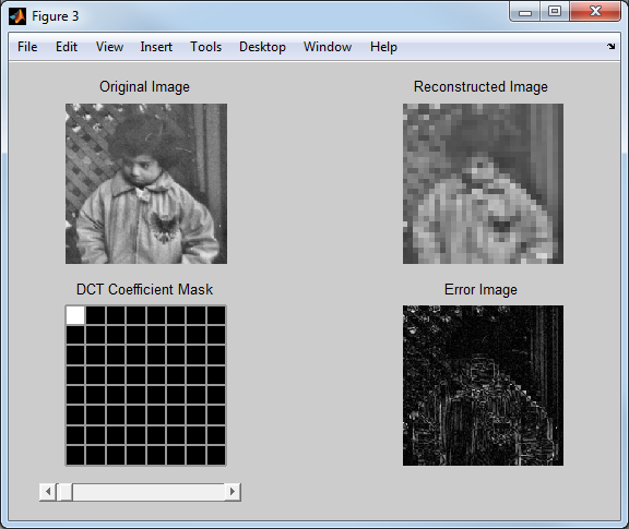
Here's the result with the DCT coefficient mask visualization included:

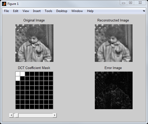
The last thing I want to do with this little app is to allow users to set the app's NumDCTCoefficients property from the command line and to have the app automatically update. To do this, I'll make a couple of changes to the NumDCTCoefficients property. First, I'll make it a dependent property. Instead of being stored independently, this property will be computed on-the-fly from slider setting whenever it is queried. That requires that I define a property get method that computes the property's value on demand. And last I'll need a property set method that defines what actions should be taken whenever the user sets the property.

Here's the modified property block that indicates that NumDCTCoefficients is a dependent property.

properties (Dependent)
    NumDCTCoefficients
end

And here are the get and set functions for NumDCTCoefficients. The get function computes the number on-the-fly based on the current slider position. The set function modifies the slider position and then calls the update method to recompute and redisplay everything.

function value = get.NumDCTCoefficients(app)
    value = round(get(app.Slider,'Value') * 64);
end

function set.NumDCTCoefficients(app,num_coefficients)
    set(app.Slider,'Value',num_coefficients/64)
    update(app);
end

Here's an example of this interaction.

app = dctCompressionExample_v5

app = 

  dctCompressionExample_v5 with properties:

         OriginalImage: [240x240 double]
    ReconstructedImage: [240x240 double]
            ErrorImage: [240x240 double]
    DCTCoefficientMask: [8x8 logical]
    NumDCTCoefficients: 3

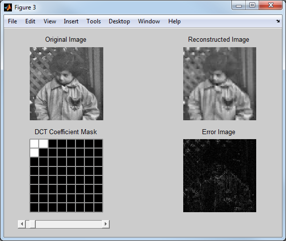
I can see the DCT coefficient mask on the app, but I can also look at the DCTCoefficientMask property.

app.DCTCoefficientMask

ans =

     1     1     0     0     0     0     0     0
     1     0     0     0     0     0     0     0
     0     0     0     0     0     0     0     0
     0     0     0     0     0     0     0     0
     0     0     0     0     0     0     0     0
     0     0     0     0     0     0     0     0
     0     0     0     0     0     0     0     0
     0     0     0     0     0     0     0     0

And I can set the NumDCTCoefficients property, which causes the app to update.

app.NumDCTCoefficients = 1;

OK, I think that's enough to get all the basic ideas. If you want to play around with the final version of the code for this blog post, you can download it from here.

Get the MATLAB code

Published with MATLAB® R2013a

Published with MATLAB® R2013a