Image processing with a GPU

著者 Steve Eddins, December 10, 2013

11 ビュー (過去 30 日間) | 0 いいね | 8 コメント

I'd like to welcome guest blogger Anand Raja for today's post. Anand is a developer on the Image Processing Toolbox team. -Steve

Many desktop computers and laptops now come with fairly powerful Graphics Processing Units (GPU's). Initially, GPU's were mostly used to power computations for graphics applications, but soon people realized that they are just as useful for any kind of numerical computing.

GPU's are made of a large number of processing units which by themselves aren't very powerful, but become formidable when used in tandem. So, if you have processing to be done that is parallelizable, the GPU will be a great fit.

With that in mind, isn't it almost obvious that image processing is a great fit for GPU's! A lot of image processing algorithms are data-parallel, meaning the same task/computation needs to be performed on many elements of the data. Lots of image processing algorithms either operate on pixels independantly or rely only on a neighborhood around pixels (like image filtering).

So, lets get down to it. My desktop computer has a GPU, and I want to do some image processing using my favorite software (no prizes for guessing), MATLAB. Note that in order to interact with the GPU from MATLAB, you require the Parallel Computing Toolbox.

I can use the gpuDevice function to get information about my GPU.

gpuDevice

ans = 

  CUDADevice with properties:

                      Name: 'Tesla C2075'
                     Index: 1
         ComputeCapability: '2.0'
            SupportsDouble: 1
             DriverVersion: 5.5000
            ToolkitVersion: 5
        MaxThreadsPerBlock: 1024
          MaxShmemPerBlock: 49152
        MaxThreadBlockSize: [1024 1024 64]
               MaxGridSize: [65535 65535 65535]
                 SIMDWidth: 32
               TotalMemory: 5.6368e+09
                FreeMemory: 5.5362e+09
       MultiprocessorCount: 14
              ClockRateKHz: 1147000
               ComputeMode: 'Default'
      GPUOverlapsTransfers: 1
    KernelExecutionTimeout: 0
          CanMapHostMemory: 1
           DeviceSupported: 1
            DeviceSelected: 1

Seeing that I have a supported GPU, I can read an image and transfer the image data to my GPU using the constructor for the gpuArray class. The gpuArray object is used to access and work with data on the GPU.

im = imread('concordaerial.png');
imGPU = gpuArray(im);
imshow(imGPU);

So imGPU is a gpuArray object containing data of type uint8.

class(imGPU)
classUnderlying(imGPU)

ans =

gpuArray


ans =

uint8

A number of the functions in the Image Processing Toolbox have support for GPU processing in R2013b. This means you can accelerate existing MATLAB scripts and functions with minimal changes. To find the list of functions that are supported for GPU processing in the Image Processing Toolbox, you can visit this page. Some of the basic image processing algorithms like image filtering, morphology and edge detection have GPU support and this list is going to grow in the coming releases.

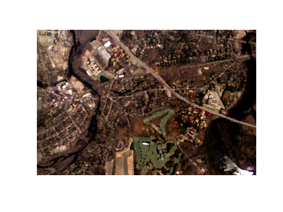
Let's look at a small example to set the ball rolling. Inspired by Brett Schoelson's guest post a few months back about Photoshop-like effects in MATLAB, I thought I might do one of my own. I call it the canvas effect . The canvas effect gives an image the feel of a canvas painting. I had created this little function that does it.

type canvasEffect

function out = canvasEffect(im)

% Filter the image with a Gaussian kernel.
h = fspecial('gaussian');
imf = imfilter(im,h);

% Increase image contrast for each color channel.
ima = cat( 3, imadjust(imf(:,:,1)), imadjust(imf(:,:,2)), imadjust(im(:,:,3)) );

% Perform a morphological closing on the image with a 11x11 structuring
% element.
se = strel('disk',9);
out = imopen(ima,se);

It's fairly straight-forward. I first smooth the image with a Gaussian kernel to round off some edges. Then to give the effect of more vivid colors, I increase the contrast for each color channel and finally a morphological opening gives it the canvas painting look. Ofcourse, you could add more bells and whistles by providing additional inputs for the filter kernel size and structuring element, but I wanted to keep it simple.

The script below reads an aerial image and gives it that canvas painting effect.

type canvasAerialCPU

% Read the image.
im = imread('concordaerial.png');

% Produce canvas effect.
canvas = canvasEffect(im);

%Display the canvas-ed image.
figure; imshow(canvas);

All the processing in the script above was done on the CPU. To move the computation to the GPU, I need to transfer the image from the CPU to the GPU using the gpuArray constructor. So the new script would like this:

type canvasAerialGPU

run canvasAerialGPU

% Read the image.
im = imread('concordaerial.png');

% Transfer data to the GPU.
imGPU = gpuArray(im);

% Produce canvas effect.
canvasGPU = canvasEffect(imGPU);

% Gather data back from the GPU.
canvas = gather(canvasGPU);

%Display the canvas-ed image.
figure; imshow(canvas);

Wasn't that easy! All I had to do was convert the image to a gpuArray and gather data back after all the computation was done. The function canvasEffect did not have to change at all. This was because all functions used in canvasEffect were supported for GPU computing.

Let's see how much of a win this is in terms of performance. For a few years now I've been using the timeit function that Steve put on the File Exchange. From R2013b, the timeit function is part of MATLAB.

cpuTime = timeit(@()canvasEffect(im), 1)

cpuTime =

    3.1311

This function however can only be used to benchmark computations undertaken by the CPU. For the GPU, a special benchmarking function gputimeit has been provided. This function ensures that all computations have completed on the GPU before recording the finish time.

gpuTime = gputimeit(@()canvasEffect(imGPU), 1)

gpuTime =

    0.2130

So with these small changes, I was able to get a considerable speed-up. Imagine having to do this on an entire data set of images. Working with the GPU would save a lot of processing time.

speedup = cpuTime/gpuTime

speedup =

   14.6990

This is not the complete picture though. I have not accounted for the time it takes to transfer data from the CPU to the GPU and back. This may or may not be significant, depending on how long the computations themselves take. As a rule of thumb, minimize data transfers to and from the device.

transferTimeToGPU = gputimeit(@()gpuArray(im), 1)
transferTimeToCPU = gputimeit(@()gather(canvasGPU), 1)

gpuTime = transferTimeToGPU + gpuTime + transferTimeToCPU;

speedup = cpuTime/gpuTime

transferTimeToGPU =

    0.0037


transferTimeToCPU =

    0.0074


speedup =

   13.9753

I'm going to end with some pointers about the performance of GPU processing.

We've seen in the simple example above that you can get a significant speed-up using the supported functions. However, this speed-up is highly dependent on your hardware. If you have a very capable CPU with multiple cores and a not-so-good GPU, the speed-up can appear to be poor because functions like imfilter and imopen are multi-threaded on the CPU. Similarly, if you have a reasonable GPU on a not-so-capable CPU, you're speed-up can make you're GPU execution look faster than it is.
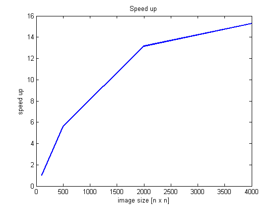
The speed-up achieved is dependent on image size. At smaller image sizes, the overhead of parsing input arguments and moving data to and from the GPU contribute to lower speed-ups. Here's an example that demonstrates this.

% Define image sizes over which to measure performance.
sizes = [100 500 2000 4000];

% Preallocate timing arrays.
[cpuTime,gpuTime,transferTimeToGPU,transferTimeToCPU] = deal(zeros('like',sizes));

for n = 1 : numel(sizes)
    size = sizes(n);

    % Resize image to size x size.
    im_scaled = imresize(im,[size size]);

    % Transfer resized image to GPU.
    imGPU_scaled = gpuArray(im_scaled);

    % Process image on GPU.
    canvasGPU_scaled = canvasEffect(imGPU_scaled);

    % Time CPU execution.
    cpuTime(n)           = timeit(@()canvasEffect(im_scaled), 1);

    % Time GPU execution.
    transferTimeToGPU(n) = gputimeit(@()gpuArray(im_scaled)       , 1);
    gpuTime(n)           = gputimeit(@()canvasEffect(imGPU_scaled), 1);
    transferTimeToCPU(n) = gputimeit(@()gather(canvasGPU_scaled)  , 1);
end

gpuTotalTime = transferTimeToGPU+gpuTime+transferTimeToCPU;
% Plot CPU vs GPU execution
figure;
plot(sizes, cpuTime, 'rx--',...
     sizes, gpuTotalTime,'bx--',...
     'LineWidth',2);
legend('cpu time','gpu time');
xlabel('image size [n x n]');
ylabel('execution time');
title('cpu time vs gpu time');

figure;
plot(sizes,cpuTime./gpuTotalTime,'LineWidth',2);
xlabel('image size [n x n]');
ylabel('speed up');
title('Speed up');