Making Color Spectrum Plots – Part 2
It was a while ago now, but on April 27 I started explaining how I made this plot, which is from DIPUM3E (Digital Image Processing Using MATLAB, 3rd ed.):
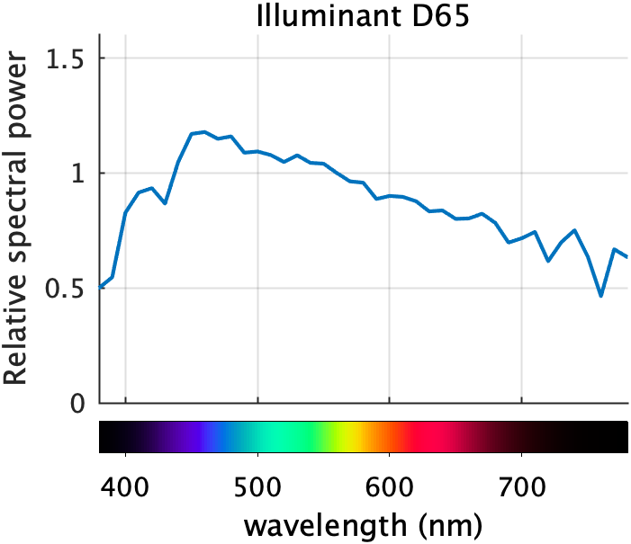
In today's follow-up, I'll discuss how I computed the colors of the spectrum to display below the x-axis. I will use and refer to several DIPUM3E functions. These are available to you in MATLAB Color Tools on the File Exchange and on GitHub. The entire set of DIPUM3E functions is also on GitHub.
Contents
Visible wavelength
What should the x-axis limits be on this plot? In other words, what is the visible wavelength that we are interested in? You will see different limits being used in different places. The limits used here, 380 nm to 780 nm, are those given in Berns, R. S. (2000). Billmeyer and Saltzman's Principals of Color Technology, 3rd ed., John Wiley & Sons, NJ.
lambda = 380:780;
Find XYZ values for the spectral colors
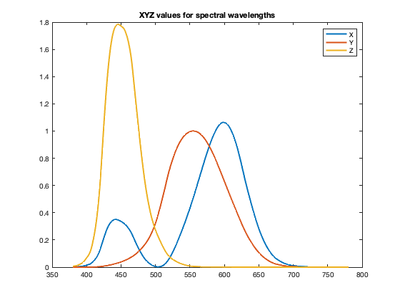
The first computational step is to find the XYZ values for each value of lambda. This computation can be found in the DIPUM3E function lambda2xyz. But it is really simple: just interpolate into the CIE XYZ color matching functions, which are returned by the DIPUM3E function colorMatchingFunctions.
T = colorMatchingFunctions;
head(T)
ans =

  8×4 table

    lambda        x             y             z
    ______    __________    __________    __________

     360       0.0001299     3.917e-06     0.0006061
     361      0.00014585    4.3936e-06    0.00068088
     362       0.0001638    4.9296e-06    0.00076515
     363        0.000184    5.5321e-06    0.00086001
     364      0.00020669    6.2082e-06    0.00096659
     365       0.0002321     6.965e-06      0.001086
     366      0.00026073    7.8132e-06     0.0012206
     367      0.00029308    8.7673e-06     0.0013727
To find the XYZ values for a specific lambda, such as 500, we can use interp1:
interp1(T.lambda,[T.x,T.y,T.z],500)
ans =

    0.0049    0.3230    0.2720
Or we can find the XYZ values for all of the wavelengths we are interested in.
XYZ = interp1(T.lambda,[T.x,T.y,T.z],lambda(:));
plot(lambda(:),XYZ)
title("XYZ values for spectral wavelengths")
legend("X","Y","Z")
Try a simple XYZ to RGB conversion
Let's try simply converting these XYZ values directly to RGB using the Image Processing Toolbox function xyz2rgb.
RGB = xyz2rgb(XYZ);
drawColorbar(RGB)

(The function drawColorbar is below. It uses the DIPUM3E function colorSwatches.)
That doesn't look like a very good spectral color plot to me. It seems uneven, with several patches that seem to be mostly one color. What's going on with this? We can see the problem if we draw a line plot of the RGB values. (The plotrgb and shadeGamutRegion functions are down below.)
close
plotrgb(lambda(:),RGB)
shadeGamutRegion

The gray shaded region shows the range between 0 and 1; this is the displayable range of colors. Everything outside that range (negative values, or values greater than 1), can't be displayed exactly. These out-of-range values are being clipped to the displayable range, and that leads to a bad results.
I'm going to show you the method used by the DIPUM3E function spectrumColors. The method is a variation of the one described in: Andrew Young (2012). Rendering Spectra (https://aty.sdsu.edu/explain/optics/rendering.html). Retrieved July 16, 2020.
Work with linear RGB values
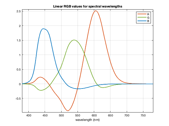
First, let's convert the XYZ values to "linear" RGB values. The typical RGB values we see for image pixels are related nonlinearly to light intensity, and linear RGB values are more appropriate for the following averaging and scaling steps. The Image Processing Toolbox function xyz2rgb can optionally convert to linear values.
RGB_lin = xyz2rgb(XYZ,'ColorSpace','linear-rgb');
plotrgb(lambda(:),RGB_lin)
title("Linear RGB values for spectral wavelengths")
Heuristic scaling of linear RGB values
We want to modify those curves so that they fall within the range [0,1] and produce a reasonably accurate, smoothly varying, and attractive representation of the spectral colors.
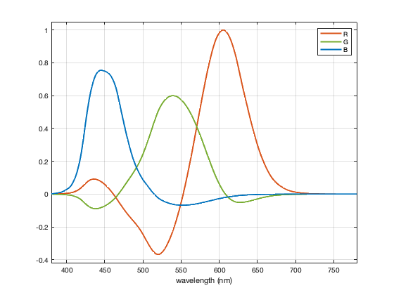
The next thing we'll do is scale so that the maximum linear RGB value is 1.0. (Note: Young (2012) divides by a fixed value of 2.34.)
RGB_lin = RGB_lin / max(RGB_lin(:));

plotrgb(lambda(:),RGB_lin)
Now, one component at a time, and for each spectral color, mix in a sufficient amount neutral gray with the same Y to bring negative component values up to 0.
Y = XYZ(:,2);
for k = 1:3
   C = RGB_lin(:,k);
   F = Y ./ (Y - C);

   % No scaling is needed for component values that are already
   % nonnegative.
   F(C >= 0) = 1;

   RGB_lin = Y + F.*(RGB_lin - Y);
end

plotrgb(lambda(:),RGB_lin)
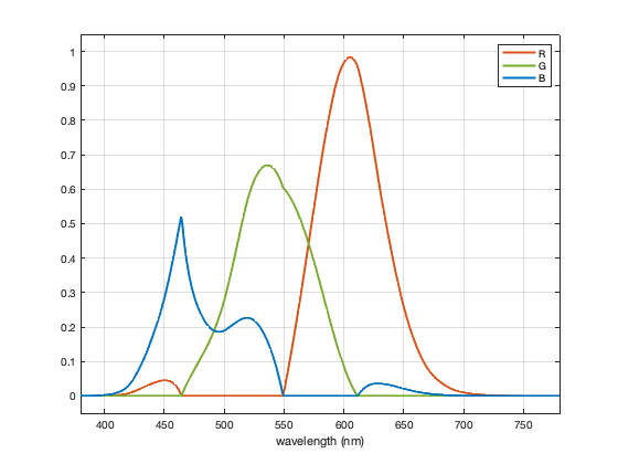
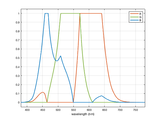
Next, to get brighter spectral colors, including a good yellow, scale up the linear RGB values, allowing them to get higher than 1.0. Then, for each color, scale all components back down, if necessary, so that the maximum component value is 1.0. Note: [Young 2012] uses a scale factor of 1.85.
RGB_lin = RGB_lin * 2.5;
S = max(RGB_lin,[],2);
S = max(S,1);
RGB_lin = RGB_lin ./ S;

plotrgb(lambda(:),RGB_lin)
Smooth the curves
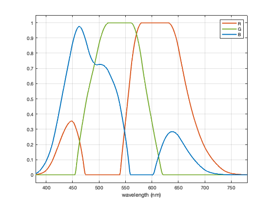
Smooth out the linear RGB curves to eliminate discontinuous first derivatives. This helps the spectrum to appear smoother, reducing sharp transition points. Note: This step is not in [Young 2012].
RGB_lin = conv2(RGB_lin,ones(21,1)/21,'same');
plotrgb(lambda(:),RGB_lin)

Eliminate small negative numbers and numbers slightly greater than 1 that have been introduced through floating-point round-off.
RGB_lin = min(max(RGB_lin,0),1);
Convert to nonlinear RGB values for the final result
Convert to nonlinear sRGB values suitable for display on a computer monitor.
RGB = lin2rgb(RGB_lin);

plotrgb(lambda(:),RGB)
drawColorbar(RGB)

Next time, I'll talk about how to draw the spectral color scale underneath the plot.
Utility functions
function drawColorbar(rgb_colors)
f = figure;
f.Position(4) = f.Position(4) / 5;
colorSwatches(rgb_colors,0)
daspect([40 1 1])
axis off
end

function plotrgb(x,rgb_colors)
% Pick the colors we want to use from the normal line color order.
c = lines(7);
blue = c(1,:);
red = c(2,:);
green = c(5,:);
clf
plot(x,rgb_colors(:,1),'Color',red);
hold on
plot(x,rgb_colors(:,2),'Color',green);
plot(x,rgb_colors(:,3),'Color',blue)
hold off
grid on
axis tight
yl = ylim;
ylim([min(yl(1)-0.05,-0.05) max(yl(2)+0.05,1.05)])

legend("R","G","B")
xlabel("wavelength (nm)")

end

function shadeGamutRegion
xl = xlim;
xx = [xl(1) xl(2) xl(2) xl(1) xl(1)];
yy = [0 0 1 1 0];
p = patch(xx,yy,[0.5 0.5 0.5],"FaceAlpha",0.1,...
    "EdgeAlpha",0.1,"HandleVisibility","off");
end


Comments
To leave a comment, please click here to sign in to your MathWorks Account or create a new one.