So, we hear you are competing in a boat competition in Hawaii? Really cool location for a competition! But wow, that’s a hard environment to replicate! Waves, ocean winds, transporting a 16-foot-long boat, not a great situation to be in! As a result, most teams have a hard time doing much controller or system testing in between those rare ocean test days.

Open Source Robotics Foundation (OSRF) has created a ROS package for simulating the conditions of the competition environment called Virtual Maritime RobotX Challenge (VMRC). The goal of the VMRC project is to help teams use simulation to design robust and thoroughly tested systems. They plan to conduct a virtual competition in 2019 based on this simulation package. This ROS package contains the following:

• Plant Model of a 16’ WAM-V Unmanned Surface Vessel
• Environment Models, e.g., water and wind physics, course elements
• Sensor Models, e.g., camera, lidar, GPS

Check out their Bitbucket repository to see how you can install and get started with this package!

All right, there’s our plant, sensor, and environment models. Now to design our controller! Simulink is a popular environment used by controls engineers in industry to design controllers. My colleague Gillian Rosen put together a simulation harness to show teams how to use Simulink to get started with doing just that. You can download the files from the MATLAB Central File Exchange. Handing over to Gillian to talk about her work!

Step 1: Connect to VMRC

As we touched on before, VMRC has a bunch of elements that simulate the competition environment and, like most ROS simulation packages, uses Gazebo as the physics engine. Naturally, our first step is: get on the ROS network and get chatting with Gazebo. If you are not familiar with using MATLAB, Simulink and ROS together, check out this blog post. After you have downloaded the File Exchange entry follow the steps in README.pdf to connect to the VMRC simulator. Some considerations:

1. The File Exchange entry has been tested in MATLAB R2018a. We will soon add support for later versions of MATLAB.
2. Ensure the environment variables are set up correctly if you are using a virtual machine in setupScript.m, especially the ROS master and ROS IP addresses. Refer to README.pdf for specific instructions.
3. VMRC uses a few custom ROS messages, such as usv_gazebo_plugins/UsvDrive, which bundles together left and right thrust commands. These will have to be registered with MATLAB as custom messages so that MATLAB can understand them. You can get all the details here.
4. For listening and talking through Simulink, you can use the ROS Subscribe and ROS Publish blocks. The data goes in and out of the blocks using a bus signal that mimics the structure of the ROS message type.

IN:

OUT:

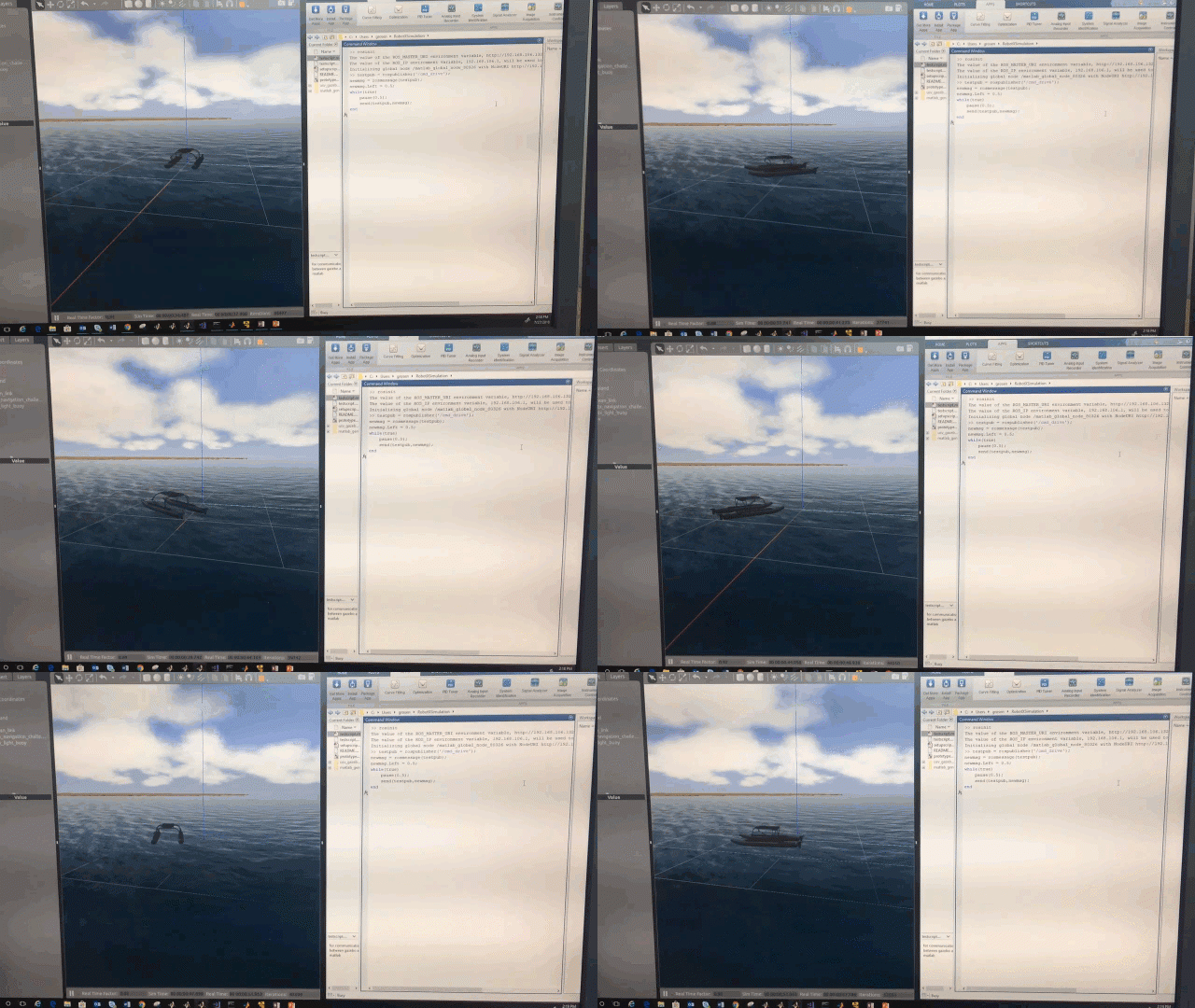
Now that you are connected to the ROS network, PERFORM WAM-V DONUTS!!!

testpub = rospublisher('/cmd_drive');
newmsg = rosmessage(testpub);
newmsg.Left = 0.5
while(true)
pause(0.3);
send(testpub,newmsg);
end

Step 2: Tackle Those Tasks

Note: VMRC strongly recommends that you have a “Discrete Graphics Card, e.g. Nvidia GTX 650” for running VMRC. I developed this model using a virtual machine running Ubuntu 16.04. It was choppy (frame rate between 1-2 Hz) but still usable.

The RobotX competition consists of a few complicated tasks that are designed to simulate popular autonomous system behavior. I’m certainly not entering the competition solo, and that’s not the point of this blog post. The point is to give:

• A foundation that you can use for communication and mission planning
• A few basic ideas for getting started on the tasks.

I picked a few tasks to focus on: Demonstrate Navigation and Control, Scan the Code, and Avoid Obstacles.

Demonstrate Navigation and Control – The Mandatory Task

Planner subchart: Navigation

I understand why this is mandatory. If you can’t drive forward 10m in a straight line, then maybe it’s not a good idea to try the other tasks.

My basic plan here was: Drive forward. While driving, use my camera to see if my alignment between the buoys is too off, and correct as necessary. Stop when I don’t see any more buoys.

The first part I tackled was finding the location of the buoys in the camera image. Connell had a color detection algorithm designed in Simulink that I used – it’s a subsystem that thresholds the camera image, does some blob wrangling, and outputs the number of blobs and the centroid of the largest blob. Subsystems (and other features, like model references) in Simulink can help with integration of independently-developed models, which is useful when you have several teams working on different aspects of a system. With one subsystem configured for red and one for green, I used the number of blobs and the relative positions of the largest blobs of each color to determine how well-aligned I was.

For correcting as necessary, I used a simple bang-bang controller: turn left, turn right, go straight, or stop. Since I was going to need to use these directions in multiple contexts, I made a “Directions” enumeration so that I didn’t have to remember “0 = straight”, “1 = left”, etc. – I got MATLAB to remember it for me.  I turned the directions into thrust commands with a bit of Stateflow logic captured as a graphical function.

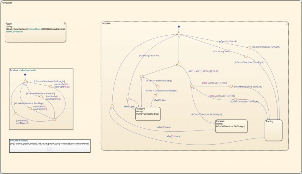
When I didn’t see any green or red buoys any more, I stopped. I noticed that the WAMV stopped a little short of the end buoys if it stopped immediately after losing sight of the buoys, so I added 10 seconds of driving straight to get me to the finish line. I stayed stopped until I spotted a buoy again.

Scan the Code

Planner subchart: ScanTheCode

My basic plan here was: identify the current buoy color with my camera. Keep watching the colors change until I see a valid sequence of three colors.

Thanks again to Connell for that color detector! I tore it apart a little to make it work for this task.  The camera image arrives from Gazebo in RGB format, so I converted it to HSV to make thresholding more straightforward (and improve performance a bit).  To get the threshold values for each color, I grabbed screenshots of the video feed with the buoy showing each color, then went to the Color Thresholder app to determine the values for each color.

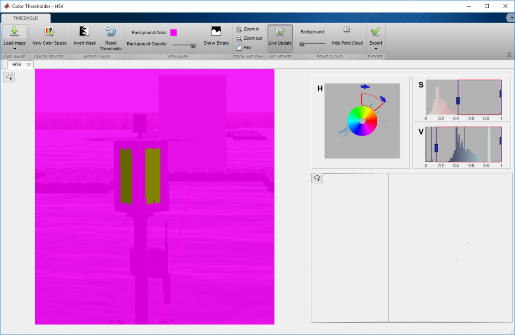
The app can export a MATLAB function with the current limits for each channel, so I looked into the code of the generated function to find my minimum and maximum values. Using the corresponding values for each color, I thresholded the Saturation and Value channels once, and the Hue channel four times — once for each possible code color (red, green, blue, yellow).

After obtaining the four thresholded images, I counted the number of valid pixels in each one and picked the hue with the largest number of valid pixels as the current color. Matrix math and manipulation are some of MATLAB’s strengths, so I used a MATLAB Function block to do the calculations. After finding the current color, all I had to do was keep track of what I had seen until I had a valid sequence of three colors.

Unit testing is key when prototyping such systems. Take for example the Scan the Code task, with my Ubuntu VM setup, VMRC wasn’t running at top speed, and I was getting a framerate of about 0.2 Hz from my camera, so I really didn’t want to wait for the camera images to come in over the ROS network or deal with the camera’s peculiarities just to test my color detection algorithm. You will notice that the color detection algorithm is formatted as a Simulink function inside a Stateflow chart for the final model, but for initial development and testing, this task was just an ordinary Simulink subsystem as shown below. This is how you can quickly perform unit tests in Simulink.

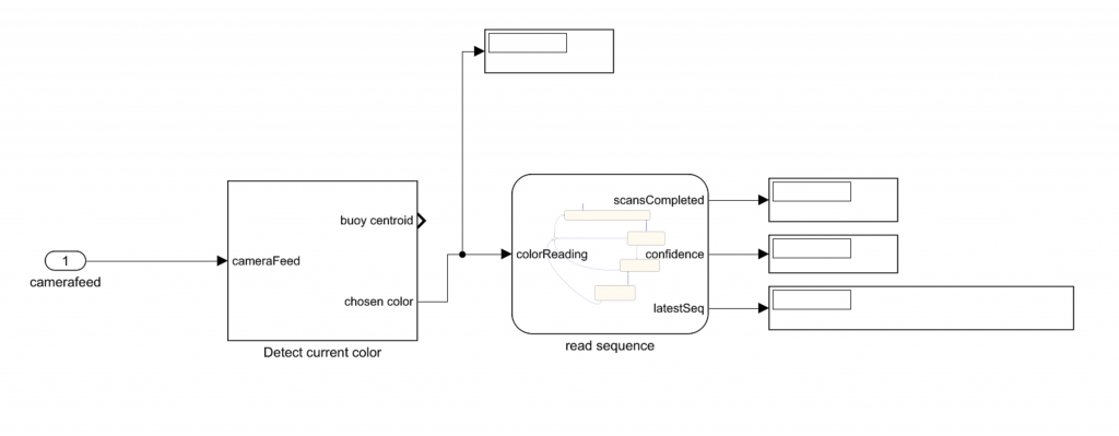
For the thresholding part, I moved the WAMV up to the buoy in Gazebo, grabbed a single camera message using the MATLAB command line, converted it to an ordinary image, and then just used it from my MATLAB workspace as a dummy camera feed.

For testing the color picker, since it’s written in a MATLAB Function block, I copied the function into a blank MATLAB script and then debugged and tested in MATLAB using my workspace image. Once I was done working on it, I just copied the updated function back into the MATLAB Function block.

For testing the sequence-reading logic in the Stateflow chart, I leaned on Stateflow animation to track what was happening in the chart. This was the one place where the slow speed of my VMRC simulation was helpful. Stateflow highlighted the state I was currently in, and I could watch the chart transition between states to trace the logic.

I just used my eyes with some display blocks and signal value labeling to test, but if you’re looking for more rigorous and scalable options, check out Simulink Design Verifier.

Avoid Obstacles

Planner subchart: ObstacleAvoidance

My basic plan here was to use the LiDAR scans and the Vector Field Histogram (VFH) obstacle avoidance block from the Robotics System Toolbox. The WAM-V’s lidar scan comes in as a 3D point cloud of XYZ points and the VFH block takes a 2D scan in range/angle format. I figured I could take a slice of the point cloud at a certain height to create a 2D scan, then convert the XY points of the 2D scan to ranges and angles. The WAM-V’s lidar scan was tilted by roughly 20 degrees. This meant that I couldn’t just slice the scan at a certain Z-coordinate. I needed to align the pointcloud to the ground plane, so back to MATLAB to prototype the matrix math. I converted the XYZ coordinates to spherical, estimated the most common elevation angle, and rotated the pointcloud accordingly.

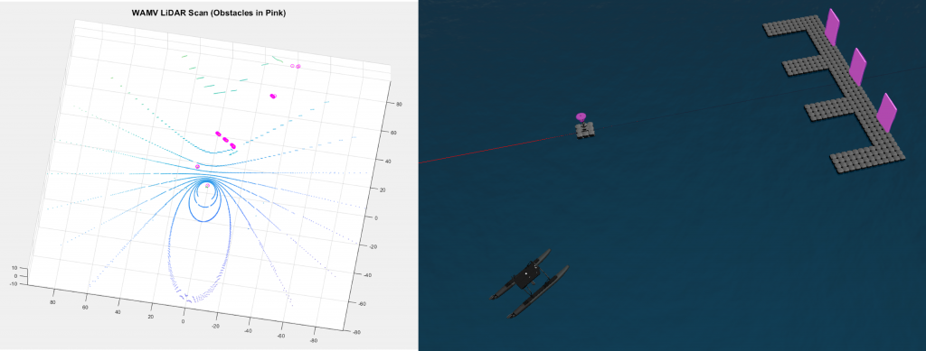
To move these calculations into the model, I used a combination of an Interpreted MATLAB Function block and a MATLAB Function block. The two blocks both let you run MATLAB functions within Simulink, but they have some differences in functionality due to how they run the code. I settled on using the Interpreted MATLAB block for the affine transformation, then sending the transformed pointcloud to the MATLAB Function block for generating the ranges and angles.

Step 3: Put Them Together

Once all the individual task controllers were completed and tested, I moved them into one big Stateflow chart. Each task is contained in a subchart with two parallel states, plus all the MATLAB, Simulink, and graphical functions needed to support those two states. One state extracts the necessary data from the ROS data input bus and processes it for the other state to use, and the second tracks/updates the current state and assigns outputs.  The data-processing state goes first, but both states are executed at each time step.

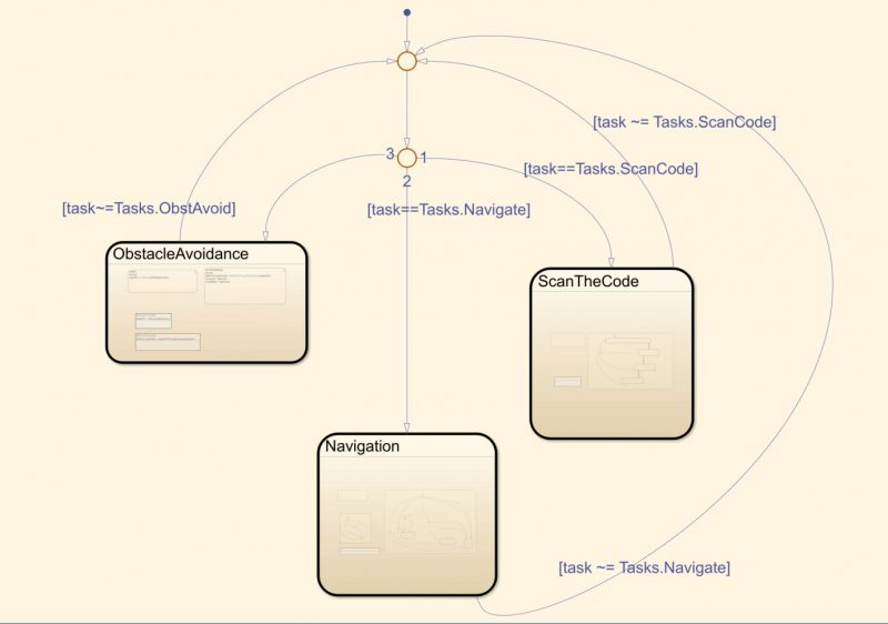
The top level selects the current task. In the model, the current task is controlled by flipping manual switches, but you could use real logic just as well. I used just one single bus for the input instead of individual inputs for each sensor so that I could switch my sensor configuration when needed. The bus definition is saved in the MATLAB workspace so that if I say “my ROS data bus”, Simulink or Stateflow can just go look it up instead of having it hard-coded. If I decide that I want to use another camera or that I don’t want to use the GPS any more, all I have to do is add/delete the subscribers I want and update the bus definition.

When authoring state charts in text-based programming languages, having all the actual logic three indents deep because of all your control flow is bad enough, but having logic that you only want to do upon entry/exit to a state is not trivial. I’ve tried adding mini-states that just lead into or out of the main state or flags and conditional logic to check if a state is being entered for the first time. Stateflow has this: (example link)

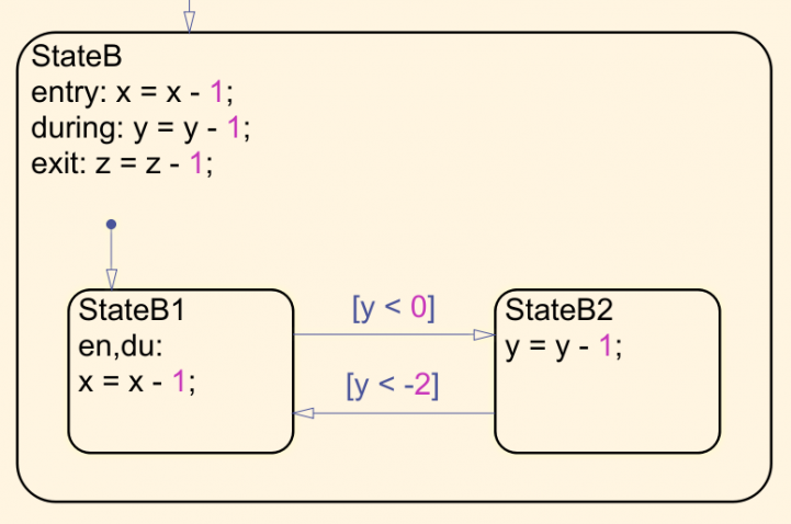
If there’s something that you only want to do on entry, put it after an entry: in the state contents. To understand how Stateflow charts are executed take a look at this documentation page.

Wrapping up

That’s the model! There you have it! With what you’ve seen in this blog, you have a good foundation to:

• Connect MATLAB and Simulink to the VMRC simulation
• Use Stateflow (which is very cool) for high-level mission planning as well as for individual tasks
• Integrate algorithms written in Simulink and MATLAB with charts written in Stateflow

After prototyping your controller with Simulink, you can generate code from the model to deploy it directly to your system, or you can generate a ROS Node to use it with VMRC. For more info on code generation, check out this video series, which is made specifically for student competitions.

Good luck!