
Building Regression Models: A Tutorial for the WiDS Datathon 2022
Introduction
Hello! I am Grace Woolson, an Application Support Engineer at the MathWorks. We are excited to support the Women in Data Science Datathon 2022 by providing complimentary MATLAB Licenses, tutorials, and resources to each participant.

This tutorial will walk you through the steps of solving a regression problem with MATLAB for any dataset, while showing examples for each step using a sample dataset. Even after the Datathon has concluded, you can continue to use this blog and any linked resources to learn more about machine learning and regression with MATLAB. Please note that this blog post is an executable MATLAB Live Script, so you have the opportunity to run the code in this tutorial in your browser using MATLAB Online or download the script and run it on a local MATLAB installation. You can find these options at the bottom of the tutorial.
To request complimentary licenses for you and your teammates, go to this MathWorks site, click the “Request Software” button, and fill out the software request form.
The WiDS Datathon 2022 focuses on mitigating climate change by identifying the energy consumption of buildings through data created in collaboration with Climate Change AI (CCAI) and Lawrence Berkeley National Laboratory (Berkeley Lab). Brought to you by the WiDS Worldwide team and Harvard University IACS, the Datathon will run until February 26th, 2022. Learn more about the WiDS Datathon, or register to participate today.
The Datathon task is to train a model that predicts building energy consumption based on regional differences in building energy efficiency, as this could help determine the best targets for retrofitting. Since the model will be predicting a building’s energy consumption, which is a quantitative result, this problem could be solved using a regression model.

Before you get started with this tutorial, please execute the following code in MATLAB if you wish to follow along with the examples. This creates the dataset that I will be using. This dataset contains information about vehicles, and we will use this dataset to create a model that predicts how many miles a vehicle can drive per gallon of gas (‘MPG’).
To execute the code in this example, you can either copy/paste the individual code snippets into the Command Window and press the ‘Enter’ key, or if you are using the live script provided with this example then clicking Run Section from the Toolstrip will execute all of the code in the current section.
load carbig
tbl = table(Acceleration, cyl4, Cylinders, Displacement, Horsepower, Mfg, Model, Model_Year, MPG, org, Origin, Weight,…
‘VariableNames’, {‘Acceleration’, ‘Cyl4’, ‘Cylinders’, ‘Displacement’, ‘Horsepower’, ‘Make’, ‘Model’, ‘Year’, ‘MPG’, ‘RegionOfOrigin’, ‘CountryOfOrigin’, ‘Weight’});
writetable(tbl, ‘carData.csv’);
clear;
clc;
After executing this, you should have a file called ‘carData.csv’ in your current directory. Now, you are ready to start building your own regression model by following the steps of the machine learning workflow.

Access and Explore the Data
Real-world data tends to come with real-world challenges. Datasets could be stored in a variety of different file types, may be stored across several files, and can get messy and confusing. In this section, I will discuss some basic steps for loading and cleaning up a dataset in MATLAB.
Step 1: Import Your Data
In order to start working with data, you have to first bring it into the Workspace. If your data is stored across multiple files, you may wish to use a datastore, as it provides a convenient way for accessing these files. It stores information about the files in a given location and the format of their contents, and only imports the files when you need them. To learn more about datastores, refer to the documentation page.
In this example, all of our data is stored in one .CSV file, so I will be importing the data as a table. Tables can store data with different data types and allow for the use of headers to label the data in a column, also called a variable, so they lend themselves nicely for storing large or complicated datasets in the workspace. To import a table from a file, you can either use the Import Tool or the ‘readtable’ command.
Option 1: Using the Import Tool
The Import Tool lets users preview and import data interactively, without having to write any code. To open the Import Tool, navigate to the Toolstrip at the top of the MATLAB window, click on the Home tab, find the ‘Variable’ section, and click Import Data. This will open a window that prompts you to select the file you wish to import; after you have selected a file, it will open the Import Tool.
From here, you can see the data in the file, each variable name, and the data type of each variable. Additionally, you can set import options and declare how to treat cells that cannot be imported. I will use the default settings, and click Import Selection to finish importing the data.
The Import Tool can also be opened by executing the following command in the Command Window:
uiimport(‘carData.csv’);
Option 2: Using Commands
Importing data using the ‘readtable’ command means that you won’t get a preview of the data before you import it, but it may be more helpful if you wish to customize the import options beyond what the Import Tool offers. For example, this command may be preferred if the data has multiple indicators to say that a value is missing.
In our example, ‘carData.csv’ always uses NaN when a value is missing, which is automatically interpreted by MATLAB as a missing value. Let’s say, however, that we are working with a dataset called ‘messyData.csv’ that uses NaN, ‘-‘, ‘NA’, -99, and ‘.’ to indicate when there is missing data. In this case, you could use the ‘TreatAsMissing’ Name-Value argument available with ‘readtable’ to convert all of these to NaN:
importedData = readtable(‘messyData.csv’, ‘TreatAsMissing’, {‘-‘, ‘NA’, ‘-99’, ‘.’});
To learn more about the options available when using ‘readtable’ to import data, please visit this documentation site.
Preprocess the Data
Now that you have the data in the Workspace, it is time to prepare it for machine learning. It is important that the data is in the correct format and that the values are what you expect them to be, as this can prevent error messages and poor model performance later on in the workflow.
Step 2: Clean Data
As I mentioned above, data is messy. Datasets may be missing entries, they may have thousands of rows or observations, they could utilize a variety of data types, the measurements may not have been taken in perfect conditions, and the data collected may not be equally representative of all possible inputs. Before you can create a model, it is important to clean the data up so that it accurately reflects the problem and can easily be used as input to train the model.
There are many different approaches you can take to work with missing values and inconsistent data. I will go through some basic steps in this post, but you can also refer to this documentation page to learn more.
First, I use the ‘summary’ function to learn more about the data types and get basic statistics about the data for each variable.
summary(carData)
Once you have learned more about the data, you can begin to think of ways to clean it up. Do you want to convert character arrays to numerical arrays, or do you want to ignore the character arrays completely? How are you going to handle missing values? What about categorical arrays? What if the minimum or maximum value of a variable seems like it is much lower or higher than it should be? Depending on the data you are working with, the answers to these questions may be different. Here are the topics I considered when cleaning up ‘carData’ before using it to create a model.
Remove the String and Categorical Variables
Some algorithms that can be used to train regression models only allow for numeric values, so I removed any non-numeric and categorical variables.
carData = removevars(carData, {‘Cyl4’, ‘Make’, ‘Model’, ‘RegionOfOrigin’,…
‘CountryOfOrigin’})
Handle Missing Data
When it comes to missing data, there are three things you should ask yourself.
- What values are used to indicate that a piece of data is missing?
- Is there a good way to fill in the missing data, or should I leave it as missing?
- Under what circumstances should I delete an observation with missing data?
What values are used to indicate that a piece of data is missing?
If your data has multiple missing value indicators and you did not import your data with the ‘TreatAsMissing’ option mentioned earlier, you can handle these missing value indicators at this step. The ‘standardizeMissing’ function allows users to easily convert custom missing value indicators to the standard missing value in MATLAB. For numeric values and durations, this standard value is NaN; for datetime values, it is NaT.
‘carData’ only uses NaN to represent a missing value, so we do not need to modify anything in this step. Let’s say, however, that we are working with ‘messyData.csv’ again, but this time it has already been imported as a table in the variable ‘messyData’. As a reminder, the person who made this dataset used NaN, ‘-‘, ‘NA’, -99, and ‘.’ to indicate when there is missing data. To quickly standardize these missing value indicators, we can use the ‘standardizeMissing’ command as follows:
standardizedData = standardizeMissing(messyData,{‘-‘, ‘NA’, -99, ‘.’});
Is there a good way to fill in the missing data, or should I leave it as missing?
With some datasets, there may be a good way to approximate the value of a missing entry, and if you do not have a lot of data to work with, it may be important to try to fill in these gaps.
One way to do this is to calculate simple statistics, such as the mean, median, or mode, of a given variable and replace all missing values in the variable with the result. This method is particularly effective if the values are similar. If the variable is increasing or decreasing in a linear fashion, then another way to fill a missing entry could be to approximate the value based on the neighboring values.
In MATLAB, the easiest way to fill missing entries is to use the ‘fillmissing’ function. It allows you to easily approximate and fill in missing values by indicating how you would like the values to be filled. Continuing the example from the previous section, let’s say that ‘standardizedData’ has a variable called ‘Age’ that seems to be increasing in a linear fashion, but it is missing some values. These values could easily be filled by executing the following command:
standardizedData.Age = fillmissing(standardizedData.Age, ‘linear’);
While there are certainly benefits to filling in missing values, doing so can get complicated and may result in poor performance of the model if the approximations are not representative of the actual data. Since our dataset only has a few missing values, I will be leaving these as NaN.
Under what circumstances should I delete an observation with missing data?
The answer to this depends on a lot of things: How much data do you have to work with? How many missing values are there? What variables have the most missing data? If you have a lot of data available, it may make sense to delete any observations with missing data. If the dataset is missing a lot of entries, maybe you choose to only delete observations with 15 or more missing values.
Before we can decide what to do, we need to know what is missing. Let’s take a look at the observations in ‘carData’ that are missing any entries:
% Get indices of all missing values
missingIdx = ismissing(carData);
% Get indices of any rows that contain missing values
rowIdxWithMissing = any(missingIdx, 2);
% Return rows with missing values
rowsWithMissing = carData(rowIdxWithMissing, : )
As you can see, ‘carData’ does not have a lot of missing data, but we do not have an abundance of observations to work with either. Some of the missing values are in the ‘MPG’ variable, which is the value that we want our model to predict. Since we cannot train a model without a predictor variable, I delete all observations that are missing the ‘MPG’ value, but leave the other missing values.
carData = rmmissing(carData, ‘DataVariables’, ‘MPG’)
Finalize the data
At this point, ‘carData’ should have 7 variables left: ‘Acceleration’, ‘Cylinders’, ‘Displacement’, ‘Horsepower’, ‘Year’, ‘MPG’, and ‘Weight’. Since ‘MPG’ is our predictor variable, I will move this to be the last column in the table.
carData = movevars(carData, “MPG”, “After”, “Weight”)
This is because many of MATLAB’s machine learning tools assume that the final variable in an input table will be the predictor, so by moving this now it makes it easier for us to work with the data in the future.
Step 3: Create Training and Testing Data
No matter what format your data is in, it is important to have separate training and testing data. Training data is fed to the model, which “teaches” the model how to predict the output value; the testing data is sent to the model after it has already been trained to see how well it performs on new data. Often, it is also beneficial to have validation data, which is used during training to prevent overfitting.
Overfitting is when the model learns the training data so well that it is able to predict the output of the training data with a high level of accuracy, but performs poorly when predicting the output for any other data. This could be caused by a number of things, including a lack of diversity in the training data. If we trained our car model on only 4 cylinder cars from the early 90’s, for example, the model would likely learn how to predict the miles per gallon for those cars very well, but would not be able to do so for any other type of vehicle. Validation data may be excluded from training data and is used to intermittently test the overall performance of the model, as this provides an idea of what the model’s overall accuracy may be.
Separate the dataset
Many of MATLAB’s tools use sections of the training data to perform validation, so I will only be creating a training set and a testing set. When creating these different datasets, it is important to try to ensure that both sets contain a variety of data to avoid bias and overfitting. If your data represents buildings, ensure it has data for different types of buildings. If it represents patients, include various ages, races, and previous health history. If it is images, include different angles and lighting. In this case, ‘carData’ is sorted by Year, so if I were to just split the data in half, both sets of data would be missing any cars from several years. Instead, I separate the data by intervals.
% every third observation is used for testing
testIdx = 1:3:398;
testData = carData(testIdx, : )
% the rest is used for training. Remove testing data from trainData
trainData = carData;
trainData(testIdx, : ) = []
It is up to you to determine how you will split the data between training and testing. A common starting point uses approximately 80% of the data for training and 20% for testing. In this example, since we only have 398 observations, I split it up so that 66% of the dataset is used for training and 33% is used for testing.
Separate the Predictor Variable from the Testing Data
Once I have a testing set, I remove the predictor variable ‘MPG’ from the table and store it in its own variable. This will make it easier to evaluate the model’s performance later.
testAnswers = testData.MPG;
testData = removevars(testData, “MPG”)
If the data you are working with was already separated into training and testing sets, then this step should be relatively simple. Make sure you have imported and cleaned up both sets of data, and then remove the predictor variable from the testing set and save it in a different variable.
Train a Model
Now that the data has been prepared, it is time to start training a model! I will be showing how to use the Regression Learner app to create a model, but I will also include examples at the bottom of this section that showcase programmatic workflows for creating a model if you want to learn more about these options. Additionally, if you would like to watch a video overview of the Regression Learner app, you can find one for a different dataset here!
Step 4: Train Models using the Regression Learner App
The Regression Learner App lets you interactively train, validate, and tune different regression models. Here is how I create a model that will predict a vehicle’s miles per gallon based on our data:
1. Open the App: On the ‘Apps’ tab, in the ‘Machine Learning and Deep Learning’ section, click Regression Learner.
Alternatively, you can open the Regression Learner app from the command line:
regressionLearner
2. Start a New Session: Click New Session and select your training data from the workspace. Specify the response variable.
3. Choose a Validation Method: Select the validation method you want to use to avoid overfitting. You should see three options: Cross-Validation, Holdout Validation, and Resubstitution Validation. I chose Cross-Validation for this example, but for problems where you have a large amount of data to work with you may wish to choose Holdout Validation. You can refer to this documentation page to learn more about these validation methods.
4. Click Start Session
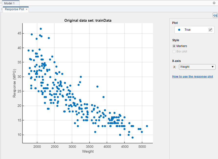
5. Investigate Variable-Response Relationships: Use the response plot to investigate which variables are useful for predicting the response. To visualize the relationship between different predictor variables and the response variable (‘MPG’), select different variables in the ‘X’ list under ‘X-axis’. Observe which variables are correlated most clearly with the response. Displacement, Horsepower, and Weight all have a visible impact on the response and all show a negative association with the response.
6. Select Model(s): On the ‘Regression Learner’ tab, in the ‘Model Type’ section, select the algorithm to be trained. I have chosen to train All, so that I can see which model type performs the best on the data.
7. Tune parameters: The Regression Learner app enables users to specify certain preferences when training a model. Options in the ‘Features’ section allow you to choose which variables are used to train the model or to enable principal component analysis (PCA). Parameters can be further adjusted by selecting a model in the ‘Models’ window and then clicking on Advanced in the ‘Regression Learner’ tab. To learn more about the advanced options for each model type, please refer to this documentation page.
Since we are creating our first model, I will be leaving the parameters as their default values.
8. Click Train.
9. Investigate Model Performance: Once the models have finished training and validation, the ‘Models’ window on the left displays the trained models and their root mean square error (RMSE). Notice that Model 1.18 has the lowest RMSE, and that the value is highlighted to indicate this. Please note: the numbers you see may be a little different.
In addition to the RSMEs, you can measure the results of training by creating visuals through the ‘Plots’ section of the ‘Regression Learner’ tab. The ‘Validation Results’ section of the drop down menu allows you to plot the relationships between predicted ‘MPG’ of the validation data and the actual ‘MPG’ of the validation data for any trained model. Simply click on the model you want to evaluate, then click on the type of plot you want to see!
To learn more about assessing a model from within the app, please refer to this documentation page.
10. Choose a Model: For this example, I will be using Model 1.18 that we trained in the previous step.
Step 5: Export your Model
Once you have tested different settings and found a model that performs well, export the model to the Workspace by selecting Export Model from the Regression Learner app. This will allow you to make predictions on the test set. I used the default name ‘trainedModel’ when exporting.
As can be seen below, the exported model is actually a structure containing the model object as well as some additional information about the model, or metadata. Since the model I have exported is a Gaussian Process model, the model object is stored in the ‘RegressionGP’ property of ‘trainedModel’. If you have exported a different type of model, this property will be called something different. You can learn the name of the propety that contains your model object by executing the following command and identifying what property replaces ‘RegressionGP’ for your model.
trainedModel
So, if I need to access the model object without any of the metadata, I can execute the following:
trainedModel.RegressionGP
Examples: Using Custom Algorithms
If you have some experience with regression learning, then you may wish to also explore programmatic options for developing a regression model. I have included some example workflows below that may help you get started. These workflows could be done instead of or in addition to using the regression learner app.
- Linear Regression Workflow
- Nonlinear Regression Workflow
- Linear Mixed-Effects Model Workflow
- All MATLAB Regression Examples
Additionally, if you create a model in the Regression Learner app, you have the option to export the code that generates your model by clicking on Generate Function from within the ‘Export’ section. This is a good way to learn about the programmatic workflow that creates a model you have trained using the app.
Evaluate Your Model
Once you have a model in the Workspace, you should evaluate it against the test data to see how the model performs on data that it has not seen. There are many ways to evaluate a model’s performance, and in this section I will show how to collect some numeric and visual measurements of a model’s performance. If you are interested in learning more about other functions that can aid in assessing a model’s performance, please refer to the relevant ‘Diagnostics’ section within this documentation page
Step 6: Collect Statistical Measurements
The following code returns the predicted responses to the new test data:
predictedMPG = trainedModel.predictFcn(testData)
If you created your model programmatically, then you would need to use the syntax below:
predictedMPG = predict(trainedModel, testData);
Using these predictions, we can take a look at the model’s performance from a few different perspectives. First, it will be helpful to calculate the error, or the difference between the actual ‘MPG’ value and the predicted ‘MPG’ value, for each observation in the test set:
testErrors = testAnswers – predictedMPG
In many cases, the array of error values will be too large to read through every single entry, and even if we did, it would be difficult to draw any meaningful conclusions. A simple measure of error may be to determine the average error value:
testAvgError = sum(abs(testErrors)) ./ length(testAnswers)
Unfortunately, this does not tell us anything about the distribution of error, so it is not really representative of the performance of our model. The ‘loss’ function calculates the loss or mean squared error of a model, which is the result of the equation below:
myLoss = sum(testErrors .* testErrors) ./ length(testErrors)
Mean squared error is more representative of the performance of a model than the average error. This is because if all of the errors are relatively low, then the loss will be low as well, but even if there are only a few predictions with a large error, then when these error values are squared they will become a much larger number. The loss is therefore increased more to represent these few predictions with a high degree of error, which is not something that calculating the average error takes into account.
The ‘loss’ function only takes the model object, not the other metadata that is stored in the ‘trainedModel’ variable, so we must extract the model object before we calculate the loss.
trainedModel.RegressionGP;
testLoss = loss(trainedModel.RegressionGP, testData, testAnswers)
Now you can compare this value to the calculated loss on the training data. Does it perform about the same, better, or much worse?
trainLoss = loss(trainedModel.RegressionGP, trainData, trainData.MPG)
In this case, the loss for the testing set is 10.1686, but it is only 1.6916 for the training set! This is an indicator that the model is overfitting. This likely means that there is data in the test set that is not represented well in the training set, so the model is not trained on how to handle these inputs yet. Changing the training and testing sets and altering the ratio of each may help improve the model’s performance.
Step 7: Create Visual Measurements
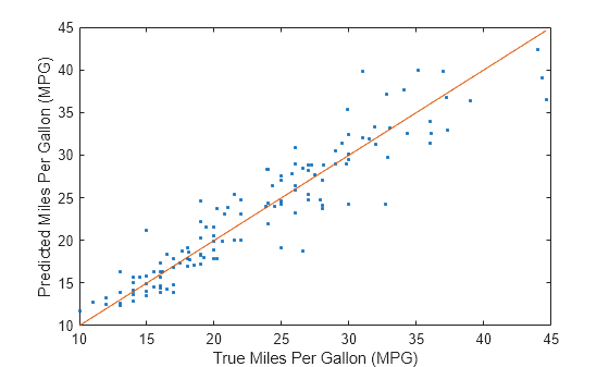
In addition to calculating these statistics, it is often beneficial to create visuals that reflect the performance of the model. The following code plots a solid line representing the actual ‘MPG’ of the test data, then adds a scatter plot representing the predicted values corresponding to each actual value. The further away a point is from the solid line, the less accurate the prediction was.
plot(testAnswers, testAnswers);
hold on
plot(testAnswers, predictedMPG, “.”);
hold off
xlabel(‘Actual Miles Per Gallon’);
ylabel(‘Predicted Miles Per Gallon’);

While many of the points are pretty close to the line, there are a few that deviate from it pretty heavily, especially as the actual ‘MPG’ value increases. This could indicate that the training data did not have many observations where the ‘MPG’ was above 30, so we may need to reconsider the division of the training and test sets. It is also possible that this indicates an overall lack of observations where ‘MPG’ was above 30 in ‘carData.csv’.
There are many ways to investigate the training and testing data beyond what you can learn from the ‘summary’ function. For example, if you want to investigate how many entries are above 30 in the training set:
trainAbove30 = numel(trainData.MPG(trainData.MPG > 30))
It turns out that only 54 entries, which is about 20% of the training set, is above 30. The ‘MPG’ values of ‘carData’ have a minimum of 9 and a maximum of 46.6, which results in a range of 37.6, and values above thirty would have to be between 30 and 46.6, which results in a range of 16.6. If the data were distributed evenly throughout the testing set, we would expect values above 30 to make up about 16.6/37.6 or 44% of the testing set.
Another way to visualize the performance of your model is to plot the error (also called the residual in this context) directly. To do this, you plot a horizontal line at 0, then scatter plot the residuals of the predictions relative to the actual ‘MPG’. A good model usually has residuals scattered roughly symmetrically around 0. Clear patterns in the residuals are a sign that you can improve your model.
plot(testAnswers,testErrors,“.”)
hold on
yline(0)
hold off
xlabel(“Actual Miles Per Gallon (MPG)”)
ylabel(“MPG Residuals”)

A positive residual means the predicted value was too low by that amount, and a negative residual means that the predicted value was too high by that amount. On this graph, it is easier to see that even though the errors may be greater for predictions on higher ‘MPG’ values, there are also a few predictions on lower ‘MPG’ values with a residual lower than negative 5, indicating a high degree of error. Even though both graphs help visualize errors, they offer different perspectives on them and plotting both may allow you to identify different patterns.
To learn more about the observations with the greatest residual, you can index into the testing set based on the residual. The code below returns a table with all observations where the residual is greater than five or less than negative five:
testData(testErrors > 5 | testErrors < -5, : )
There are a few elements or patterns that can be identified from this table that may have resulted in the model’s poor performance on these observations. Some of the observations are missing a ‘Horsepower’ value, four of them have a ‘Year’ of 80, two have ‘Cylinders’ values that are odd numbers which is uncommon in ‘carData’, some have a very low value in ‘Displacement’ and ‘Horsepower’, and the first observation’s weight is less than the minimum value of ‘Weight’ that appears in the training data. It is not immediately obvious why some of the observations confused the model, but if you start with the patterns that you can find then others may become more apparent over time as you fine-tune your model.
When you have identified patterns, you can create additional plots to confirm those patterns! For example, I have just noted that many of the observations in our table had a moderately low value in the ‘Displacement’ variable, so I decided to plot the residuals against their corresponding Displacement:
plot(testData.Displacement, testErrors, “.”);
hold on
yline(0)
hold off
xlabel(‘Displacement’);
ylabel(‘MPG Residuals’);

Here we can confirm that observations with a ‘Displacement’ under 200 tend to be predicted with less accuracy than those with a higher ‘Displacement’, which should prompt us to revisit our training data and parameters and adjust accordingly.
Rinse & Repeat
There is no one algorithm that suits all problems. You should create and test many different models because there are so many ways to fine tune a model, and even two models that have similar RMSE may perform better on different parts of the data. When using the Regression Learner app, do not just go with the model that performs best initially, but try changing parameters on a bunch of them. Change the training data, the validation method, the advanced options, the model type, and anything else that you come up with! Even if the change does not result in better performance, you might be able to learn something from it.
For each model you create, try asking yourself these questions:
- Does it perform better than my other models?
- What are the differences between this and my other models? What are the similarities?
- Which observations does it perform poorly on? Why?
If you have exported a model to the workspace and you wish to save it for later use or comparison, you may want to give it a descriptive name and save it to a .MAT file. To save the model I made in this example, I execute the following:
gaussianOne = trainedModel;
save gaussianOne;
This way if you clear your workspace or accidentally overwrite the ‘trainedModel’ variable, you still have the model saved. When you want to use it again, you can easily load it back into the workspace:
load gaussianOne;
Save Predictions
You may want to save your predictions for various reasons. Maybe you want to compare your results with those of a peer, perhaps you want to share them with someone who doesn’t use MATLAB, or maybe you need to submit your predictions for a datathon. Whatever the reason, saving and exporting your results can be done in a few easy steps.
First, since ‘carData’ did not come with any IDs and I only want to save the predictions, not any of the data, I will add a ‘car_id’ column to the test dataset:
% Create array of IDs, turn into column array using ‘ operator.
carID = (1:length(predictedMPG))’;
% Add new variable to the table at the beginning
testData = addvars(testData, carID, ‘Before’, ‘Acceleration’)
Now you can place the test results in a table containing just the ID numbers and predicted ‘MPG’ values, which makes it easy to visualize, to compare to other predictions, and to write to the desired file format.
testResults = table(testData.carID,predictedMPG,‘VariableNames’,{‘car_id’,…
‘predicted_mpg’})
Then write the results to a CSV file. This is the file type that you will submit for the WiDS Datathon challenge.
writetable(testResults,‘testResults.csv’);
All done!
Thank you for joining me on this tutorial! We are excited to find out how you will take what you have learned to create regression models that contribute to climate change research. I strongly recommend looking at the ‘Additional Resources’ section below for more ideas on how you can improve your models.
Feel free to reach out to us at studentcompetitions@mathworks.com if you have any further questions.
Further Examples
If you are interested in learning more about regression learning and other data science workflows in MATLAB, please refer to the following examples:
- This Data Science Tutorial video series will take you through a more in-depth walk through of the regression learning process when the data is stored across multiple files. This is a great example if you have the time! You can find the code in the ‘Related Resources’ section of each video if you wish to follow along.
- The Machine Learning Onramp brings you through a few classification examples and teaches the basics of machine learning with MATLAB.
- Our Deep Learning Onramp walks you through introductory deep learning methods for creating networks in MATLAB for image recongition.
- If you are interested in a more advanced regression example, this Time Series Forecasting Using Deep Learning page shows users how they can use a neural network to predict a future number of chickenpox cases.
Additional Resources
- Overview of Supervised Learning (Video)
- Missing Data in MATLAB
- Supervised Learning Workflow and Algorithms
- Train Regression Models in Regression Learner App
- Export Regression Model to Predict New Data
- 8 MATLAB Cheat Sheets for Data Science
- For a basic introduction to MATLAB: MATLAB Onramp
- MATLAB Online
Vocabulary
Observation: A row in a dataset.
Variable: A column in a dataset.
Error/Residual: The difference between an actual/expected value and the value predicted by a machine learning model. Error may be the absolute value, whereas residual must represent the distance and direction of the error.
Mean Squared Error/Loss: A value that reflects a model’s performance by squaring each prediction’s error then calculating the average of all of these values. Represented by the equation below.
myLoss = sum(testErrors .* testErrors) ./ length(testErrors)
Metadata: Additional information that is associated with an object; a set of data that provides information about other data.
- カテゴリ:
- Data Science,
- MATLAB


コメント
コメントを残すには、ここ をクリックして MathWorks アカウントにサインインするか新しい MathWorks アカウントを作成します。