
Acquiring and Analyzing Sensor Data with MATLAB Mobile and MATLAB Online
MATLAB Mobile allows you to collect information from your device sensors and perform cool experiments with the acquired data. For this post, I would like to welcome Luiz Zaniolo, our development manager to talk about one such experiment.
While I wrote this blog post, all credit for the experiment must go to my son, Giancarlo, a Carnegie Mellon University student (and adventure sports enthusiast) who wanted to perform some tests with his BMX bicycle.
His objective: determine how much time the bike spent in the air in a jump.
Acquire Sensor Data with MATLAB Mobile
His means: he used an interesting technique to attach his cell phone to the bike and turned on the accelerometer in MATLAB Mobile, started logging data, and proceed to ride the bicycle and jump over a small ramp.
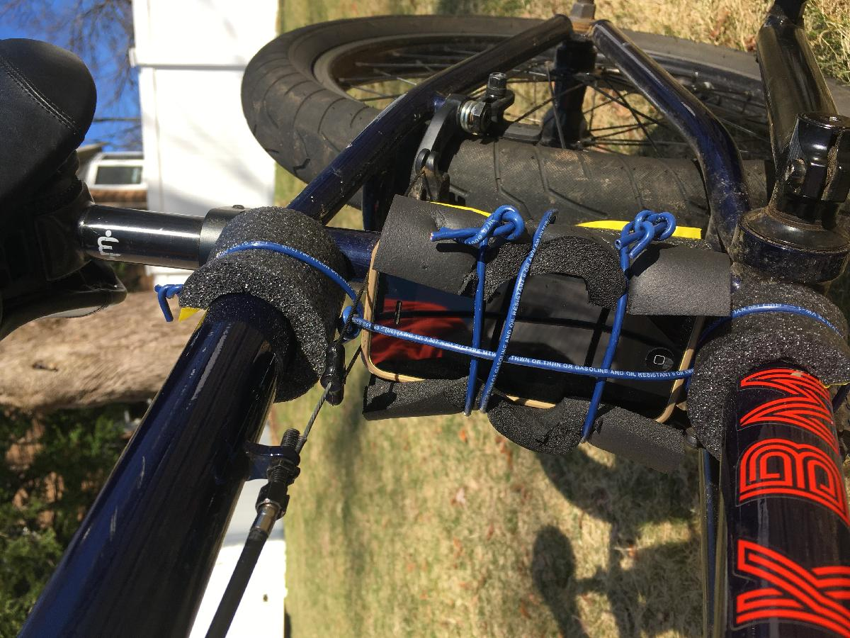
The log file was automatically uploaded to MATLAB Drive after the data collection ended.
Quick primer for those who are not aware: MATLAB Mobile can acquire data from your device sensors. You can analyze the data directly in MATLAB Mobile, MATLAB Online or on a MATLAB session on your desktop. You can even log sensor data when you are offline.
Analyze Sensor Data in MATLAB Online
Visualize Acceleration Data
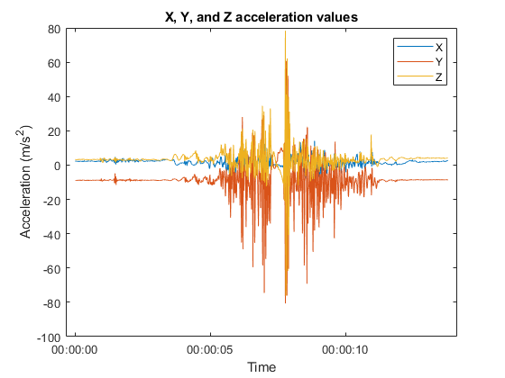
To start analyzing the data, my son logged in to MATLAB Online on his laptop, loaded the .mat file and plotted the acceleration results in the X, Y, and Z axes.
load jumpKink.mat
xAcceleration = Acceleration.X;
yAcceleration = Acceleration.Y;
zAcceleration = Acceleration.Z;
rawTimestamp = Acceleration.Timestamp;
timestamp = rawTimestamp - rawTimestamp(1);
allAxis = [xAcceleration, yAcceleration, zAcceleration];
figure; plot(timestamp, allAxis)
title('X, Y, and Z acceleration values')
xlabel('Time')
ylabel('Acceleration (m/s^2)')
legend('X', 'Y', 'Z')
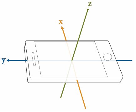
Since the measurement axis on a smartphone is defined as shown in the picture below, the most appropriate axis to measure gravity acceleration is Y.
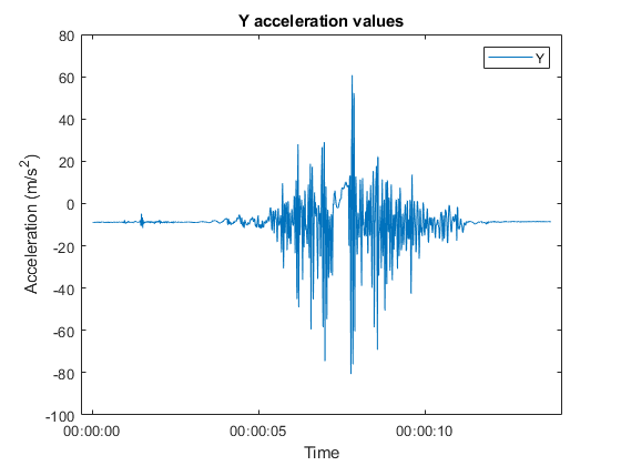
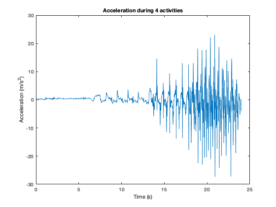
Plotting the acceleration on the Y axes gives us more clarity on the 3 different states: stopped, riding, and jumping.
figure; plot(timestamp, yAcceleration)
title('Y acceleration values')
xlabel('Time')
ylabel('Acceleration (m/s^2)')
legend('Y')
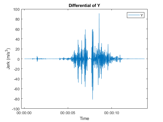
Calculate Rate of Change
By differentiating the acceleration file, he was able to identify the jerk (rate of change of acceleration), which should be small when the bike is either stopped or in the air.
difYAcceleration = diff(yAcceleration);
timestampdif = timestamp;
timestampdif(end)=[]; % remove last element to match with difYAcceleration array
figure; plot(timestampdif, difYAcceleration)
title('Differential of Y')
xlabel('Time')
ylabel('Jerk (m/s^3)')
legend('Y')
Determine "Air Time"
He then applied his algorithm to detect when the bicycle was in the air. The algorithm implements a low-pass filter in the differential signal by averaging the time measurement with 2 neighbors on each side and outputs an array of the current state in time.
% mode 0: stopped
% mode 1: riding
% mode 2: in air
modeArray = zeros(length(yAcceleration), 1);
filteredDifArray = zeros(length(difYAcceleration), 1);
modeArray(1) = 0;
airCounter = 0;
threshold = 16;
for i = 3 : (length(difYAcceleration) - 2)
sumOfPoints = abs(difYAcceleration(i-2)) + abs(difYAcceleration(i-1)) + ...
abs(difYAcceleration(i)) + abs(difYAcceleration(i+1)) + abs(difYAcceleration(i+2));
filteredDifArray(i) = sumOfPoints / 5;
% if it passes the threshold (moving on bumpy enough ground)
if sumOfPoints > threshold
% if in "air" for less than 0.25 secs before jump lands, read over all "air"s with 1s
if airCounter < 25
for j = i : -1 : (i - airCounter)
modeArray(j) = 1;
end
end
modeArray(i) = 1;
airCounter = 0;
elseif sumOfPoints < threshold
% if it doesnt pass the threshold (either still or in air)
if modeArray(i - 1) == 0 || length(yAcceleration) - i < 300
%if its stopped it stays stopped
modeArray(i) = 0;
%if its still for too long it counts it as stopped, reads over all "air"s with 0s
elseif airCounter >= 300
for j = i: -1: (i - airCounter)
modeArray(j) = 0;
end
else
modeArray(i) = 2;
end
airCounter = airCounter + 1;
end
end
Finally, plotting the mode array on top of the Y acceleration shows the detections of different modes: stopped, riding, and jumping.
modeArray = modeArray .* 20; % amplify to show better in graph scale
figure; plot(timestamp, yAcceleration)
hold on
plot(timestamp, modeArray, 'r')
hold off
title('Jump Detection Algorithm')
xlabel('Time')
ylabel('Acceleration (m/s^2)')
legend('Y', 'modeArray')
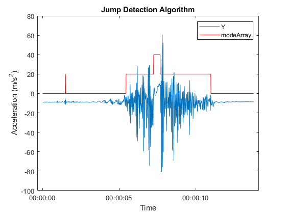
And since he had the mode array, he counted how many samples were reported as "in air" to display the total air time of 0.44 seconds.
numOfAirSamples = sum (modeArray == 40);
airTime = numOfAirSamples * 0.01 % the acquisition rate was 100 samples per second
Tell Us About Your Experiments!
Even though this is a simple example of signal processing, my son described it as something that he enjoyed doing. The intermediate plots helped him understand better what needed to be done to accomplish his task. Although if he's planning to execute more reckless jumps to improve his air time, his father needs to have a talk with him.
Have you used your phone to collect sensor data for experiments like this? If you did, we would love to learn more. Please share them with us by adding a comment below.
- 类别:
- MATLAB Mobile


评论
要发表评论,请点击 此处 登录到您的 MathWorks 帐户或创建一个新帐户。