
Defining Your Own Network Layer
Note: Post updated 27-Sep-2018 to correct a typo in the implementation of the backward function.
One of the new Neural Network Toolbox features of R2017b is the ability to define your own network layer. Today I'll show you how to make an exponential linear unit (ELU) layer.
Joe helped me with today's post. Joe is one of the few developers who have been around MathWorks longer than I have. In fact, he's one of the people who interviewed me when I applied for a job here. I've had the pleasure of working closely with Joe for the past several years on many aspects of MATLAB design. He really loves tinkering with deep learning networks.
Joe came across the paper "Fast and Accurate Deep Network Learning by Exponential Linear Units (ELUs)," by Clevert, Unterthiner, and Hichreiter, and he wanted to make an ELU layer using R2017b.
$f(x) = \left\{\begin{array}{ll} x & x > 0\\ \alpha(e^x - 1) & x \leq 0 \end{array} \right.$
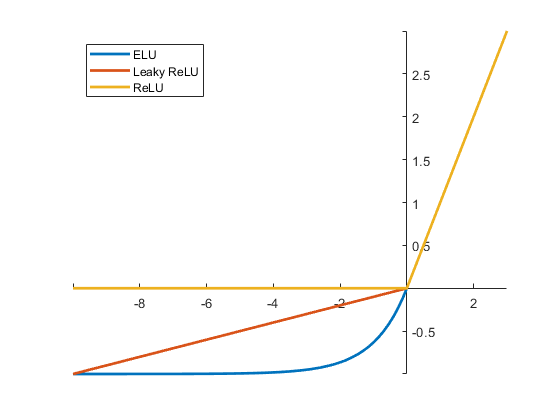
Let's compare the ELU shape with a couple of other commonly used activation functions.
alpha1 = 1;
elu_fcn = @(x) x.*(x > 0) + alpha1*(exp(x) - 1).*(x <= 0);

alpha2 = 0.1;
leaky_relu_fcn = @(x) alpha2*x.*(x <= 0) + x.*(x > 0);

relu_fcn = @(x) x.*(x > 0);

fplot(elu_fcn,[-10 3],'LineWidth',2)
hold on
fplot(leaky_relu_fcn,[-10 3],'LineWidth',2)
fplot(relu_fcn,[-10 3],'LineWidth',2)
hold off
ax = gca;
ax.XAxisLocation = 'origin';
ax.YAxisLocation = 'origin';
box off
legend({'ELU','Leaky ReLU','ReLU'},'Location','northwest')
Joe wanted to make a ELU layer with one learned alpha value per channel. He followed the procedure outlined in Define a Layer with Learnable Parameters to make an ELU layer that works with the Neural Network Toolbox.
Below is the template for a layer with learnable parameters. We'll explore how to fill in this template to make an ELU layer.
classdef myLayer < nnet.layer.Layer

    properties
        % (Optional) Layer properties

        % Layer properties go here
    end

    properties (Learnable)
        % (Optional) Layer learnable parameters

        % Layer learnable parameters go here
    end

    methods
        function layer = myLayer()
            % (Optional) Create a myLayer
            % This function must have the same name as the layer

            % Layer constructor function goes here
        end

        function Z = predict(layer, X)
            % Forward input data through the layer at prediction time and
            % output the result
            %
            % Inputs:
            %         layer    -    Layer to forward propagate through
            %         X        -    Input data
            % Output:
            %         Z        -    Output of layer forward function

            % Layer forward function for prediction goes here
        end

        function [Z, memory] = forward(layer, X)
            % (Optional) Forward input data through the layer at training
            % time and output the result and a memory value
            %
            % Inputs:
            %         layer  - Layer to forward propagate through
            %         X      - Input data
            % Output:
            %         Z      - Output of layer forward function
            %         memory - Memory value which can be used for
            %                  backward propagation

            % Layer forward function for training goes here
        end

        function [dLdX, dLdW1, ..., dLdWn] = backward(layer, X, Z, dLdZ, memory)
            % Backward propagate the derivative of the loss function through
            % the layer
            %
            % Inputs:
            %         layer             - Layer to backward propagate through
            %         X                 - Input data
            %         Z                 - Output of layer forward function
            %         dLdZ              - Gradient propagated from the deeper layer
            %         memory            - Memory value which can be used in
            %                             backward propagation
            % Output:
            %         dLdX              - Derivative of the loss with respect to the
            %                             input data
            %         dLdW1, ..., dLdWn - Derivatives of the loss with respect to each
            %                             learnable parameter

            % Layer backward function goes here
        end
    end
end
For our ELU layer with a learnable alpha parameter, here's one way to write the constructor and the Learnable property block.
classdef eluLayer < nnet.layer.Layer

    properties (Learnable)
        alpha
    end

    methods
        function layer = eluLayer(num_channels,name)
            layer.Type = 'Exponential Linear Unit';

            % Assign layer name if it is passed in.
            if nargin > 1
                layer.Name = name;
            end

            % Give the layer a meaningful description.
            layer.Description = "Exponential linear unit with " + ...
                num_channels + " channels";

            % Initialize the learnable alpha parameter.
            layer.alpha = rand(1,1,num_channels);
        end
The predict function is where we implement the activation function. Remember its mathematical form:
$f(x) = \left\{\begin{array}{ll} x & x > 0\\ \alpha(e^x - 1) & x \leq 0 \end{array} \right.$
Note: The expression (exp(min(X,0)) - 1) in the predict function is written that way to avoid computing the exponential of large positive numbers, which could result in infinities and NaNs popping up.
        function Z = predict(layer,X)
            % Forward input data through the layer at prediction time and
            % output the result
            %
            % Inputs:
            %         layer    -    Layer to forward propagate through
            %         X        -    Input data
            % Output:
            %         Z        -    Output of layer forward function

            % Expressing the computation in vectorized form allows it to
            % execute directly on the GPU.
            Z = (X .* (X > 0)) + ...
                (layer.alpha.*(exp(min(X,0)) - 1) .* (X <= 0));
        end
The backward function implements the derivatives of the loss function, which are needed for training. The Define a Layer with Learnable Parameters documentation page explains how to derive the needed quantities.
        function [dLdX, dLdAlpha] = backward(layer, X, Z, dLdZ, ~)
            % Backward propagate the derivative of the loss function through
            % the layer
            %
            % Inputs:
            %         layer             - Layer to backward propagate through
            %         X                 - Input data
            %         Z                 - Output of layer forward function
            %         dLdZ              - Gradient propagated from the deeper layer
            %         memory            - Memory value which can be used in
            %                             backward propagation [unused]
            % Output:
            %         dLdX              - Derivative of the loss with
            %                             respect to the input data
            %         dLdAlpha          - Derivatives of the loss with
            %                             respect to alpha

            % Original expression:
            % dLdX = (dLdZ .* (X > 0)) + ...
            %     (dLdZ .* (layer + Z) .* (X <= 0));
            %
            % Optimized expression:
            dLdX = dLdZ .* ((X > 0) + ...
                ((layer.alpha + Z) .* (X <= 0)));

            dLdAlpha = (exp(min(X,0)) - 1) .* dLdZ;
            % Sum over the image rows and columns.
            dLdAlpha = sum(sum(dLdAlpha,1),2);
            % Sum over all the observations in the mini-batch.
            dLdAlpha = sum(dLdAlpha,4);
        end
That's all we need for our layer. We don't need to implement the forward function because our layer doesn't have memory and doesn't need to do anything special for training.
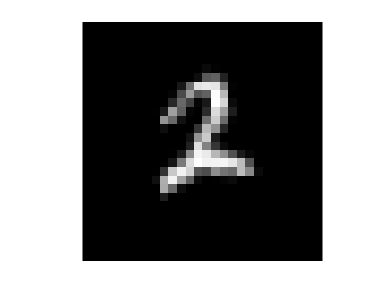
Load in the sample digits training set, and show one of the images from it.
[XTrain, YTrain] = digitTrain4DArrayData;
imshow(XTrain(:,:,:,1010),'InitialMagnification','fit')
YTrain(1010)
ans =

  categorical

     2
Make a network that uses our new ELU layer.
layers = [ ...
    imageInputLayer([28 28 1])
    convolution2dLayer(5,20)
    batchNormalizationLayer
    eluLayer(20)
    fullyConnectedLayer(10)
    softmaxLayer
    classificationLayer];
Train the network.
options = trainingOptions('sgdm');
net = trainNetwork(XTrain,YTrain,layers,options);
Training on single GPU.
Initializing image normalization.
|=========================================================================================|
|     Epoch    |   Iteration  | Time Elapsed |  Mini-batch  |  Mini-batch  | Base Learning|
|              |              |  (seconds)   |     Loss     |   Accuracy   |     Rate     |
|=========================================================================================|
|            1 |            1 |         0.03 |       2.5173 |        5.47% |       0.0100 |
|            2 |           50 |         0.63 |       0.4548 |       85.16% |       0.0100 |
|            3 |          100 |         1.20 |       0.1550 |       96.88% |       0.0100 |
|            4 |          150 |         1.78 |       0.0951 |       99.22% |       0.0100 |
|            6 |          200 |         2.37 |       0.0499 |       99.22% |       0.0100 |
|            7 |          250 |         2.96 |       0.0356 |      100.00% |       0.0100 |
|            8 |          300 |         3.55 |       0.0270 |      100.00% |       0.0100 |
|            9 |          350 |         4.13 |       0.0168 |      100.00% |       0.0100 |
|           11 |          400 |         4.74 |       0.0145 |      100.00% |       0.0100 |
|           12 |          450 |         5.32 |       0.0118 |      100.00% |       0.0100 |
|           13 |          500 |         5.89 |       0.0119 |      100.00% |       0.0100 |
|           15 |          550 |         6.45 |       0.0074 |      100.00% |       0.0100 |
|           16 |          600 |         7.03 |       0.0079 |      100.00% |       0.0100 |
|           17 |          650 |         7.60 |       0.0086 |      100.00% |       0.0100 |
|           18 |          700 |         8.18 |       0.0065 |      100.00% |       0.0100 |
|           20 |          750 |         8.76 |       0.0066 |      100.00% |       0.0100 |
|           21 |          800 |         9.34 |       0.0052 |      100.00% |       0.0100 |
|           22 |          850 |         9.92 |       0.0054 |      100.00% |       0.0100 |
|           24 |          900 |        10.51 |       0.0051 |      100.00% |       0.0100 |
|           25 |          950 |        11.12 |       0.0044 |      100.00% |       0.0100 |
|           26 |         1000 |        11.73 |       0.0049 |      100.00% |       0.0100 |
|           27 |         1050 |        12.31 |       0.0040 |      100.00% |       0.0100 |
|           29 |         1100 |        12.93 |       0.0041 |      100.00% |       0.0100 |
|           30 |         1150 |        13.56 |       0.0040 |      100.00% |       0.0100 |
|           30 |         1170 |        13.80 |       0.0043 |      100.00% |       0.0100 |
|=========================================================================================|
Check the accuracy of the network on our test set.
[XTest, YTest] = digitTest4DArrayData;
YPred = classify(net, XTest);
accuracy = sum(YTest==YPred)/numel(YTest)
accuracy =

    0.9872
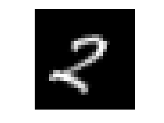
Look at one of the images in the test set and see how it was classified by the network.
k = 1500;
imshow(XTest(:,:,:,k),'InitialMagnification','fit')
YPred(k)
ans =

  categorical

     2
Now you've seen how to define your own layer, include it in a network, and train it up.
- Category:
- Deep Learning


Comments
To leave a comment, please click here to sign in to your MathWorks Account or create a new one.