
Classify ECG Signals Using LSTM Networks
Contents
- Introduction
- Load and Examine the Data
- Prepare the Data for Training
- Train the Classifier Using Raw Signal Data
- Define the LSTM Network Architecture
- Train the LSTM Network
- Visualize the Training and Testing Accuracy
- Improve the Performance with Feature Extraction
- Standardize the Data
- Modify the LSTM Network Architecture
- Train the LSTM Network with Time-Frequency Features
- Visualize the Training and Testing Accuracy
- Conclusion
- References
Introduction
ECGs record the electrical activity of a person's heart over a period of time. Physicians use ECGs to detect visually if a patient's heartbeat is normal or irregular. Atrial fibrillation (AFib) is a type of irregular heartbeat that occurs when the heart's upper chambers, the atria, beat out of coordination with the lower chambers, the ventricles. This example uses ECG data from the PhysioNet 2017 Challenge [1], [2], [3], which is available at https://physionet.org/challenge/2017/. The data consists of a set of ECG signals sampled at 300 Hz and divided by a group of experts into four different classes: Normal (N), AFib (A), Other Rhythm (O), and Noisy Recording (~). This example shows how to automate the classification process using deep learning. The procedure explores a binary classifier that can differentiate Normal ECG signals from signals showing signs of AFib. This example uses long short-term memory (LSTM) networks, a type of recurrent neural network (RNN) well-suited to study sequence and time-series data. An LSTM network can learn long-term dependencies between time steps of a sequence. The LSTM layer (lstmLayer) can look at the time sequence in the forward direction, while the bidirectional LSTM layer (bilstmLayer) can look at the time sequence in both forward and backward directions. This example uses a bidirectional LSTM layer. To accelerate the training process, run this example on a machine with a GPU. If your machine has a GPU and Parallel Computing Toolbox™, then MATLAB® automatically uses the GPU for training; otherwise, it uses the CPU.Load and Examine the Data
Run the ReadPhysionetData script to download the data from the PhysioNet website and generate a MAT-file (PhysionetData.mat) that contains the ECG signals in the appropriate format. Downloading the data might take a few minutes.ReadPhysionetData
load PhysionetData
The loading operation adds two variables to the workspace: Signals and Labels. Signals is a cell array that holds the ECG signals. Labels is a categorical array that holds the corresponding ground-truth labels of the signals.
Signals(1:5)
Labels(1:5)
ans =

  5×1 cell array

    {1×9000  double}
    {1×9000  double}
    {1×18000 double}
    {1×9000  double}
    {1×18000 double}


ans =

  5×1 categorical array

     N
     N
     N
     A
     A
Use the summary function to see that there are 738 AFib signals and 5050 Normal signals.
summary(Labels)
     A       738
     N      5050
Generate a histogram of signal lengths. Notice that most of the signals are 9000 samples long.
L = cellfun(@length,Signals);
h = histogram(L);
xticks(0:3000:18000);
xticklabels(0:3000:18000);
title('Signal Lengths')
xlabel('Length')
ylabel('Count')
 Visualize a segment of one signal from each class. AFib heartbeats are spaced out at irregular intervals while Normal heartbeats occur regularly. AFib heartbeat signals also often lack a P wave, which pulses before the QRS complex in a Normal heartbeat signal. The plot of the Normal signal shows a P wave and a QRS complex.
normal = Signals{1};
aFib = Signals{4};

subplot(2,1,1)
plot(normal)
title('Normal Rhythm')
xlim([4000,5200])
ylabel('Amplitude (mV)')
text(4330,150,'P','HorizontalAlignment','center')
text(4370,850,'QRS','HorizontalAlignment','center')

subplot(2,1,2)
plot(aFib)
title('Atrial Fibrillation')
xlim([4000,5200])
xlabel('Samples')
ylabel('Amplitude (mV)')

Prepare the Data for Training
During training, the trainNetwork function splits the data into mini-batches. The function then pads or truncates signals in the same mini-batch so they all have the same length. Too much padding or truncating can have a negative effect on the performance of the network, because the network might interpret a signal incorrectly based on the added or removed information. To avoid excessive padding or truncating, apply the segmentSignals function to the ECG signals so they are all 9000 samples long. The function ignores signals with fewer than 9000 samples. If a signal has more than 9000 samples, segmentSignals breaks it into as many 9000-sample segments as possible and ignores the remaining samples. For example, a signal with 18500 samples becomes two 9000-sample signals, and the remaining 500 samples are ignored.[Signals,Labels] = segmentSignals(Signals,Labels);
View the first five elements of the |Signals| array to verify that each
entry is now 9000 samples long.
Signals(1:5)
ans =

  5×1 cell array

    {1×9000 double}
    {1×9000 double}
    {1×9000 double}
    {1×9000 double}
    {1×9000 double}
Train the Classifier Using Raw Signal Data
To design the classifier, use the raw signals generated in the previous section. Split the signals into a training set to train the classifier and a testing set to test the accuracy of the classifier on new data. Use the summary function to show that there 718 AFib signals and 4937 Normal signals, a ratio of 1:7.summary(Labels)
     A       718
     N      4937
Because 87.3% of the signals are Normal, the classifier would learn that it can achieve a high accuracy simply by classifying all signals as Normal. To avoid this bias, augment the AFib data by duplicating AFib signals in the dataset so that there is the same number of Normal and AFib signals. This duplication, commonly called oversampling, is one form of data augmentation used in deep learning.
Split the signals according to their class.
afibX = Signals(Labels=='A');
afibY = Labels(Labels=='A');

normalX = Signals(Labels=='N');
normalY = Labels(Labels=='N');
Next, use dividerand to divide targets from each class randomly into training and testing sets.
[trainIndA,~,testIndA] = dividerand(718,0.9,0.0,0.1);
[trainIndN,~,testIndN] = dividerand(4937,0.9,0.0,0.1);

XTrainA = afibX(trainIndA);
YTrainA = afibY(trainIndA);

XTrainN = normalX(trainIndN);
YTrainN = normalY(trainIndN);

XTestA = afibX(testIndA);
YTestA = afibY(testIndA);

XTestN = normalX(testIndN);
YTestN = normalY(testIndN);
Now there are 639 AFib signals and 4441 Normal signals for training. To achieve the same number of signals in each class, use the first 4438 Normal signals, and then use repmat to repeat the first 634 AFib signals seven times. For testing, there are 71 AFib signals and 494 Normal signals. Use the first 490 Normal signals, and then use repmat to repeat the first 70 AFib signals seven times. By default, the neural network randomly shuffles the data before training, ensuring that contiguous signals do not all have the same label.
XTrain = [repmat(XTrainA(1:634),7,1); XTrainN(1:4438)];
YTrain = [repmat(YTrainA(1:634),7,1); YTrainN(1:4438)];

XTest = [repmat(XTestA(1:70),7,1); XTestN(1:490)];
YTest = [repmat(YTestA(1:70),7,1); YTestN(1:490);];
The distribution between Normal and AFib signals is now evenly balanced in both the training set and the testing set.
summary(YTrain)
summary(YTest)
     A      4438
     N      4438
     A      490
     N      490
Define the LSTM Network Architecture
LSTM networks can learn long-term dependencies between time steps of sequence data. This example uses the bidirectional LSTM layer bilstmLayer, as it looks at the sequence in both forward and backward directions. Because the input signals have one dimension each, specify the input size to be sequences of size 1. Specify a bidirectional LSTM layer with an output size of 100 and output the last element of the sequence. This command instructs the bidirectional LSTM layer to map the input time series into 100 features and then prepares the output for the fully connected layer. Finally, specify two classes by including a fully connected layer of size 2, followed by a softmax layer and a classification layer.layers = [ ... sequenceInputLayer(1) bilstmLayer(100,'OutputMode','last') fullyConnectedLayer(2) softmaxLayer classificationLayer ]
layers =

  5x1 Layer array with layers:

     1   ''   Sequence Input          Sequence input with 1 dimensions
     2   ''   BiLSTM                  BiLSTM with 100 hidden units
     3   ''   Fully Connected         2 fully connected layer
     4   ''   Softmax                 softmax
     5   ''   Classification Output   crossentropyex
Next specify the training options for the classifier. Set the '|MaxEpochs|' to 10 to allow the network to make 10 passes through the training data. A '|MiniBatchSize|' of 150 directs the network to look at 150 training signals at a time. An '|InitialLearnRate|' of 0.01 helps speed up the training process. Specify a 'SequenceLength' of 1000 to break the signal into smaller pieces so that the machine does not run out of memory by looking at too much data at one time. Set '|GradientThreshold|' to 1 to stabilize the training process by preventing gradients from getting too large. Specify 'Plots' as 'training-progress' to generate plots that show a graphic of the training progress as the number of iterations increases. Set '|Verbose|' to false to suppress the table output that corresponds to the data shown in the plot. If you want to see this table, set 'Verbose' to true.
This example uses the adaptive moment estimation (ADAM) solver. ADAM performs better with recurrent neural networks (RNNs) like LSTMs than the default stochastic gradient descent with momentum (SGDM) solver.
options = trainingOptions('adam', ...
    'MaxEpochs',10, ...
    'MiniBatchSize', 150, ...
    'InitialLearnRate', 0.01, ...
    'SequenceLength', 1000, ...
    'GradientThreshold', 1, ...
    'plots','training-progress', ...
    'Verbose',false);
Train the LSTM Network
Train the LSTM network with the specified training options and layer architecture by using trainNetwork. Because the training set is large, the training process can take several minutes.net = trainNetwork(XTrain,YTrain,layers,options);
 The top subplot of the training-progress plot represents the training accuracy, which is the classification accuracy on each mini-batch. When training progresses successfully, this value typically increases towards 100%. The bottom subplot displays the training loss, which is the cross-entropy loss on each mini-batch. When training progresses successfully, this value typically decreases towards zero.
If the training is not converging, the plots might oscillate between values without trending in a certain upward or downward direction. This oscillation means that the training accuracy is not improving and the training loss is not decreasing. This situation can occur from the start of training, or the plots might plateau after some preliminary improvement in training accuracy. In many cases, changing the training options can help the network achieve convergence. Decreasing MiniBatchSize |or decreasing |InitialLearnRate might result in a longer training time, but it can help the network learn better.
The classifier's training accuracy oscillates between 50% and 60%, and at the end of 10 epochs, it already has taken several minutes to train.
The top subplot of the training-progress plot represents the training accuracy, which is the classification accuracy on each mini-batch. When training progresses successfully, this value typically increases towards 100%. The bottom subplot displays the training loss, which is the cross-entropy loss on each mini-batch. When training progresses successfully, this value typically decreases towards zero.
If the training is not converging, the plots might oscillate between values without trending in a certain upward or downward direction. This oscillation means that the training accuracy is not improving and the training loss is not decreasing. This situation can occur from the start of training, or the plots might plateau after some preliminary improvement in training accuracy. In many cases, changing the training options can help the network achieve convergence. Decreasing MiniBatchSize |or decreasing |InitialLearnRate might result in a longer training time, but it can help the network learn better.
The classifier's training accuracy oscillates between 50% and 60%, and at the end of 10 epochs, it already has taken several minutes to train.
Visualize the Training and Testing Accuracy
Calculate the training accuracy, which represents the accuracy of the classifier on the signals on which it was trained. First, classify the training data.trainPred = classify(net,XTrain,'SequenceLength',1000);
In classification problems, confusion matrices are used to visualize the performance of a classifier on a set of data for which the true values are known. The Target Class is the ground-truth label of the signal, and the Output Class is the label assigned to the signal by the network. The axes labels represent the class labels, AFib (A) and Normal (N).
Green cells represent correctly classified signals and red cells represent incorrectly classified signals. Light gray cells provide row and column summaries. The bottom-right cell displays the overall accuracy.
plotconfusion(YTrain',trainPred','Training Accuracy')
 The confusion matrix shows that 81.7% of the ground-truth AFib signals are correctly classified as AFib, while 31.1% of ground-truth Normal signals are correctly classified as Normal. Furthermore, 54.2% of the signals classified as AFib are actually AFib, and 63.0% of the signals classified as Normal are actually Normal. The overall training accuracy is 56.4%.
Now classify the testing data.
The confusion matrix shows that 81.7% of the ground-truth AFib signals are correctly classified as AFib, while 31.1% of ground-truth Normal signals are correctly classified as Normal. Furthermore, 54.2% of the signals classified as AFib are actually AFib, and 63.0% of the signals classified as Normal are actually Normal. The overall training accuracy is 56.4%.
Now classify the testing data.
testPred = classify(net,XTest,'SequenceLength',1000);
Calculate the testing accuracy, which represents the accuracy of the classifier on new signals.
plotconfusion(YTest',testPred','Testing Accuracy')
 This confusion matrix is similar to the training confusion matrix. The overall testing accuracy is 55.8%.
Improve the Performance with Feature Extraction
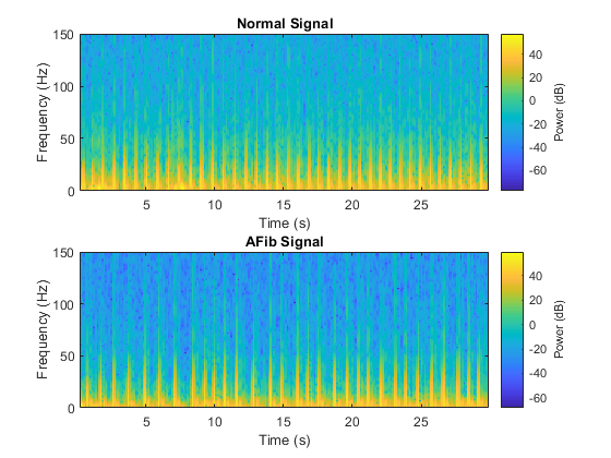
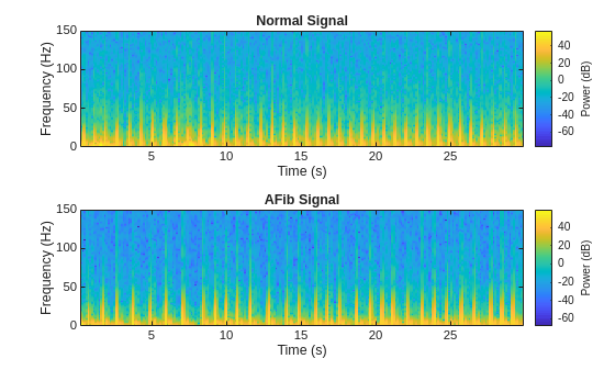
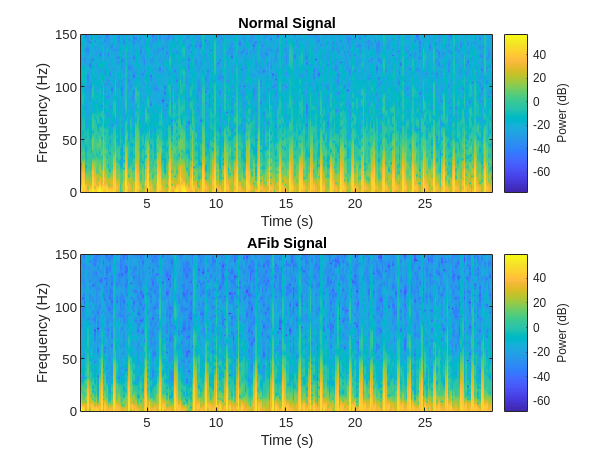
Feature extraction from the data can help improve the training and testing accuracies of the classifier. To decide which features to extract, this example follows an approach that computes time-frequency images, such as spectrograms, and uses them to train convolutional neural networks (CNNs). See [4] and [5] for more information about such applications. Visualize the spectrogram of each type of signal.fs = 300; figure subplot(2,1,1); pspectrum(normal,fs,'spectrogram','TimeResolution',0.5) title('Normal Signal') subplot(2,1,2); pspectrum(aFib,fs,'spectrogram','TimeResolution',0.5) title('AFib Signal')
 Since this example uses an LSTM instead of a CNN, it is important to translate the approach so it applies to one-dimensional signals. Time-frequency (TF) moments extract information from the spectrograms. Each moment can be used as a one-dimensional feature to input to the LSTM.
Explore two TF moments in the time domain:
Since this example uses an LSTM instead of a CNN, it is important to translate the approach so it applies to one-dimensional signals. Time-frequency (TF) moments extract information from the spectrograms. Each moment can be used as a one-dimensional feature to input to the LSTM.
Explore two TF moments in the time domain:
- Instantaneous frequency (instfreq)
- Spectral entropy (pentropy)
[instFreqA,tA] = instfreq(aFib,fs);
[instFreqN,tN] = instfreq(normal,fs);

figure
subplot(2,1,1);
plot(tN,instFreqN)
title('Normal Signal')
xlabel('Time (s)')
ylabel('Instantaneous Frequency')

subplot(2,1,2);
plot(tA,instFreqA)
title('AFib Signal')
xlabel('Time (s)')
ylabel('Instantaneous Frequency')
 Use cellfun |to apply the |instfreq function to every cell in the training and testing sets.
instfreqTrain = cellfun(@(x)instfreq(x,fs)',XTrain,'UniformOutput',false);
instfreqTest = cellfun(@(x)instfreq(x,fs)',XTest,'UniformOutput',false);
The spectral entropy measures how spiky flat the spectrum of a signal is. A signal with a spiky spectrum, like a sum of sinusoids, has low spectral entropy. A signal with a flat spectrum, like white noise, has high spectral entropy. The pentropy function estimates the spectral entropy based on a power spectrogram. As with the instantaneous frequency estimation case, pentropy uses 255 time windows to compute the spectrogram. The time outputs of the function correspond to the center of the time windows. Visualize the spectral entropy for each type of signal.
[pentropyA,tA2] = pentropy(aFib,fs);
[pentropyN,tN2] = pentropy(normal,fs);

figure

subplot(2,1,1)
plot(tN2,pentropyN)
title('Normal Signal')
ylabel('Spectral Entropy')

subplot(2,1,2)
plot(tA2,pentropyA)
title('AFib Signal')
xlabel('Time (s)')
ylabel('Spectral Entropy')
 Use cellfun |to apply the |pentropy function to every cell in the training and testing sets.
pentropyTrain = cellfun(@(x)pentropy(x,fs)',XTrain,'UniformOutput',false);
pentropyTest = cellfun(@(x)pentropy(x,fs)',XTest,'UniformOutput',false);
Concatenate the features such that each cell in the new training and testing sets has two dimensions, or two features.
XTrain2 = cellfun(@(x,y)[x;y],instfreqTrain,pentropyTrain,'UniformOutput',false);
XTest2 = cellfun(@(x,y)[x;y],instfreqTest,pentropyTest,'UniformOutput',false);
Visualize the format of the new inputs. Each cell no longer contains one 9000-sample-long signal; now it contains two 255-sample-long features.
XTrain2(1:5)
ans =

  5×1 cell array

    {2×255 double}
    {2×255 double}
    {2×255 double}
    {2×255 double}
    {2×255 double}
Standardize the Data
The instantaneous frequency and the spectral entropy have means that differ by almost one order or magnitude. Furthermore, the instantaneous frequency mean might be too high for the LSTM to learn effectively. When a network is fit on data with a large mean and a large range of values, large inputs could slow down the learning and convergence of the network [6].mean(instFreqN) mean(pentropyN)
ans =

    5.5615


ans =

    0.6326
Use the training set mean and standard deviation to standardize the training and testing sets. Standardization, or z-scoring, is a popular way to improve network performance during training.
XV = [XTrain2{:}];
mu = mean(XV,2);
sg = std(XV,[],2);

XTrainSD = XTrain2;
XTrainSD = cellfun(@(x)(x-mu)./sg,XTrainSD,'UniformOutput',false);

XTestSD = XTest2;
XTestSD = cellfun(@(x)(x-mu)./sg,XTestSD,'UniformOutput',false);
Show the means of the standardized instantaneous frequency and spectral entropy.
instFreqNSD = XTrainSD{1}(1,:);
pentropyNSD = XTrainSD{1}(2,:);

mean(instFreqNSD)
mean(pentropyNSD)
ans =

   -0.3202


ans =

   -0.2407
Modify the LSTM Network Architecture
Now that the signals each have two dimensions, it is necessary to modify the network architecture by specifying the input sequence size as 2. Specify a bidirectional LSTM layer with an output size of 100, and output the last element of the sequence. Specify two classes by including a fully connected layer of size 2, followed by a softmax layer and a classification layer.layers = [ ... sequenceInputLayer(2) bilstmLayer(100,'OutputMode','last') fullyConnectedLayer(2) softmaxLayer classificationLayer ]
layers =

  5x1 Layer array with layers:

     1   ''   Sequence Input          Sequence input with 2 dimensions
     2   ''   BiLSTM                  BiLSTM with 100 hidden units
     3   ''   Fully Connected         2 fully connected layer
     4   ''   Softmax                 softmax
     5   ''   Classification Output   crossentropyex
Specify the training options. Set the maximum number of epochs to 30 to allow the network to make 30 passes through the training data.
options = trainingOptions('adam', ...
    'MaxEpochs',30, ...
    'MiniBatchSize', 150, ...
    'InitialLearnRate', 0.01, ...
    'GradientThreshold', 1, ...
    'plots','training-progress', ...
    'Verbose',false);
Train the LSTM Network with Time-Frequency Features
Train the LSTM network with the specified training options and layer architecture by using trainNetwork.net2 = trainNetwork(XTrainSD,YTrain,layers,options);
 There is a great improvement in the training accuracy, which is now greater than 90%. The cross-entropy loss trends towards 0. Furthermore, the time required for training decreases because the TF moments are shorter than the raw sequences.
Visualize the Training and Testing Accuracy
Classify the training data. Plot the confusion matrix to examine the training accuracy. The overall training accuracy is 95.8%. Furthermore, 96.8% of AFib signals are correctly classified as AFib, and 94.7% of Normal signals are correctly classified as Normal.trainPred2 = classify(net2,XTrainSD);
plotconfusion(YTrain',trainPred2','Training Accuracy')
 Classify the testing data. Plot the confusion matrix to examine the testing accuracy. The overall testing accuracy is 93.2%. Furthermore, 94.3% of AFib signals are correctly classified as AFib, and 92.0% of Normal signals are correctly classified as Normal.
testPred2 = classify(net2,XTestSD);
plotconfusion(YTest',testPred2','Testing Accuracy')

Conclusion
This example shows how to build a classifier to detect atrial fibrillation in ECG signals using an LSTM network. The procedure uses oversampling to avoid the classification bias that occurs when one tries to detect abnormal conditions in populations composed mainly of healthy patients. Training the LSTM network using raw signal data results in a poor classification accuracy. Training the network using two time-frequency-moment features for each signal significantly improves the classification performance and also decreases the training time.References
[1] AF Classification from a Short Single Lead ECG Recording: the PhysioNet/Computing in Cardiology Challenge, 2017. https://physionet.org/challenge/2017/
[2] Clifford, Gari, Chengyu Liu, Benjamin Moody, Li-wei H. Lehman, Ikaro Silva, Qiao Li, Alistair Johnson, and Roger G. Mark. "AF Classification from a Short Single Lead ECG Recording: The PhysioNet Computing in Cardiology Challenge 2017." Computing in Cardiology (Rennes: IEEE). Vol. 44, 2017 (in press).
[3] Goldberger, A. L., L. A. N. Amaral, L. Glass, J. M. Hausdorff, P. Ch. Ivanov, R. G. Mark, J. E. Mietus, G. B. Moody, C.-K. Peng, and H. E. Stanley. "PhysioBank, PhysioToolkit, and PhysioNet: Components of a New Research Resource for Complex Physiologic Signals". Circulation. Vol. 101, No. 23, 13 June 2000, pp. e215$-$e220. <http://circ.ahajournals.org/content/101/23/e215.full
[4] Pons, Jordi, Thomas Lidy, and Xavier Serra. "Experimenting with Musically Motivated Convolutional Neural Networks". 14th International Workshop on Content-Based Multimedia Indexing (CBMI). June 2016.
[5] Wang, D. "Deep learning reinvents the hearing aid," IEEE Spectrum, Vol. 54, No. 3, March 2017, pp. 32$-$37. doi: 10.1109/MSPEC.2017.7864754.
[6] Brownlee, Jason. How to Scale Data for Long Short-Term Memory Networks in Python. 7 July 2017. https://machinelearningmastery.com/how-to-scale-data-for-long-short-term-memory-networks-in-python/.
Utility Function for this Example
function [signalsOut, labelsOut] = segmentSignals(signalsIn,labelsIn)
%SEGMENTSIGNALS makes all signals in the input array 9000 samples long


targetLength = 9000;
signalsOut = {};
labelsOut = {};

for idx = 1:numel(signalsIn)

    x = signalsIn{idx};
    y = labelsIn(idx);

    % Ensure column vector
    x = x(:);

    % Compute the number of targetLength-sample chunks in the signal
    numSigs = floor(length(x)/targetLength);

    if numSigs == 0
        continue;
    end

    % Truncate to a multiple of targetLength
    x = x(1:numSigs*targetLength);

    % Create a matrix with as many columns as targetLength signals
    M = reshape(x,targetLength,numSigs);

    % Repeat the label numSigs times
    y = repmat(y,[numSigs,1]);

    % Vertically concatenate into cell arrays
    signalsOut = [signalsOut; mat2cell(M.',ones(numSigs,1))]; %#ok<AGROW>
    labelsOut = [labelsOut; cellstr(y)]; %#ok<AGROW>
end

labelsOut = categorical(labelsOut);

end
- Category:
- Deep Learning


Comments
To leave a comment, please click here to sign in to your MathWorks Account or create a new one.