Key terms in custom training loops
In this post, I would like to go into detail on Loss, Model Gradients, and Automatic Differentiation
This is Part 2 in a series of Advanced Deep Learning Posts. To read the series, please see the following links:
- Post 1: Introduction
- Post 2: Custom Training: Key Terms (This post!)
|
In Part 1, we left off talking about the custom training loop that you need to write in order to tap into the power of the extended framework. If you have a simple network, it’s likely TrainNetwork will do the trick. For everything else, we can write the training loop ourselves.
At a high level, the training loop looks something like this:
 Key Steps in the Loop
I want to take a very simple problem to highlight the important parts of this loop, focusing on the non-optional portions in our diagram above. Our model has 2 learnable parameters, x1 and x2 and our goal is to optimize these parameters such that the output of our function is 0:
y = (x2 - x1.^2).^2 + (1 - x1).^2;
We will optimize our model till y = 0; This is a fairly classic equation (Rosenbrock) used in statistics problems. (Hint, there is a solution at x1 = 1 and x2 = 1).
We will start by guessing at the optimal solution x1 = 2, x2 = 2. This is just a starting point, and this code will show how we change these parameters to improve our model and eventually arrive at a solution.
my_x1 = 2;
my_x2 = 2;
learn_rate = 0.1;
x1 = dlarray(my_x1);
x2 = dlarray(my_x2);
[loss,dydx1,dydx2] = dlfeval(@my_loss,x1,x2);
[new_x1,new_x2] = updateModel(x1,x2,dydx1,dydx2,learn_rate);
plot(extractdata(new_x1),extractdata(new_x2),'rx');
*Do you see the correlation between this loop and deep learning? Our equation or “model” is much simpler, but the concepts are the same. We have “learnables” in deep learning such as the weights and biases. Here we have two learnable parameters here (x1 and x2). Changing the learnables in the training is what increases the accuracy of the model over time. The following training loop does the same thing as deep learning training, just a bit simpler to understand.
Let's walk through all the steps of this training loop, and point out key terms along the way.
1. Setup: Read data, convert to dlarray
dlarray is the structure designed to contain deep learning problems. This means for any "dl" functions (dlfeval, dlgradient) to work, we need to convert our data to a dlarray and then convert back using extractdata.
2. Calculate model gradients and loss
This happens in the function called my_loss:
function [y,dydx1,dydx2] = my_loss(x1,x2)
y = (x2 - x1.^2).^2 + (1 - x1).^2;
[dydx1,dydx2] = dlgradient(y,x1,x2);
end
Plugging in our values for x2 and x1, we get:
 This isn’t 0, which means we must find a new guess. The loss is the error, which we can keep track of to understand how far away we are from a good answer. Using gradient descent, a popular method to strategically update parameters, we calculate the gradient/derivative and then move in the direction opposite the slope.
To better visualize this, let's look at the quiver plot:
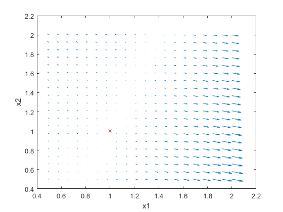 By visualizing the gradient at different points, we can see that by following the gradient, we can eventually find our way to the correct location on the plot.
The documentation for dlfeval does a great job explaining how dlgradient works, which is where I stole the quiver plot idea.
Calculate the gradient using dlgradient using automatic differentiation. This is the moment I realized automatic differentiation simply means this function is going to automatically differentiate the model, and tell us the model gradients. It's not as scary as I thought.
So from our function my_loss, we get the model gradients and loss, which are used to calculate new learnable parameters to improve the model.
3. Update the model
In our loop, the next step is to update model using the gradient to find new model parameters.
[new_x1,new_x2] = updateModel(x1,x2,dydx1,dydx2,learn_rate);
Using gradient descent, we will update these parameters, moving in the opposite direction of the slope:
function [new_x1,new_x2] = updateModel(x1,x2,dydx1,dydx2,learn_rate);
  newx1 = x1 + -dydx1*learn_rate;
  newx2 = x2 + -dydx2*learn_rate;
end
Please note, this is where this example and deep learning differ: you are not responsible for determining new learnables. This is done in the real training loop through the optimizer, ADAM or SGDM or whichever optimizer you choose. In deep learning, replace this updateModel function with SGDMUpdate or ADAMUpdate
The learning rate is how quickly you want to move in a certain direction. Higher means faster or larger leaps, but we’ll see in a second this has strong implications on how your training is going to go.
Training Loop
my_x1 = 2;
my_x2 = 2;
learn_rate = 0.1;
x1 = dlarray(my_x1);
x2 = dlarray(my_x2);
for ii = 1:100
[loss,dydx1,dydx2] = dlfeval(@my_loss,x1,x2);
[x1,x2] = updateModel(x1,x2,dydx1,dydx2,learn_rate);
plot(extractdata(x1),extractdata(x2),'bx');
end
Here is a plot of the training

After 100 iterations, we visualize the training getting closer and closer to the optimal value.
Importance of Learning Rate
As noted before, the learning rate is how quickly or how large of leaps we can take to move towards the optimal solution. A larger step could mean you arrive at your solution faster, but you could jump right over it and never converge.
Here is the same training loop above with a learn_rate = 0.2 instead of 0.1: having too high a learning rate means we could diverge and get stuck on a sub-optimal solution forever.
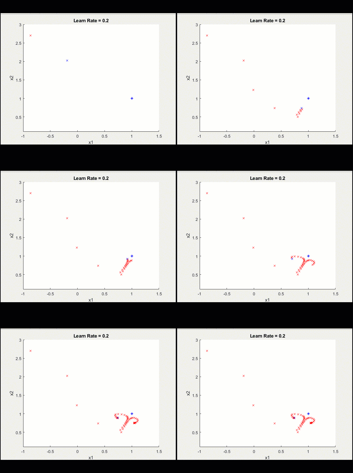
Notice this training doesn't converge toward an optimal solution, caused by a higher learning rate.
So a large learning rate can be problematic, but a smaller step could mean you are moving way too slowly (yawn), or we could end up in a local minimum, or it could take a lifetime to finish.
So, what do you do? One suggestion would be to start with a higher learning rate in the beginning, and then move to a lower learning rate as you get closer to a solution, which we can be fancy and call this "time-based decay."
Enter custom learning rates, which are simple to implement* in our custom training plot.
initialLearnRate = 0.2;
decay = 0.01;
learn_rate = initialLearnRate;
for ii = 1:100
learn_rate = initialLearnRate /(1 + decay*iteration);
end
*of course, the learning rate function could be complex, but adding it into our training loop is straightforward.
| The learning rate over the 100 iterations looks like this: |
Which causes our model to converge much more cleanly: |
 |

|
That's it! You now are fully prepared to discuss the following terms in deep learning conversations.
MATLAB functions:
- dlfeval
- dlgradient
- dlarray & extractdata
Terms:
- Automatic Differentiation:
- Loss
- Model Gradients
- Learning Rate
Resources: To prepare for this post, I went through quite a few articles in our documentation. Please look over the following links for the source material:
 Key Steps in the Loop
I want to take a very simple problem to highlight the important parts of this loop, focusing on the non-optional portions in our diagram above. Our model has 2 learnable parameters, x1 and x2 and our goal is to optimize these parameters such that the output of our function is 0:
 This isn’t 0, which means we must find a new guess. The loss is the error, which we can keep track of to understand how far away we are from a good answer. Using gradient descent, a popular method to strategically update parameters, we calculate the gradient/derivative and then move in the direction opposite the slope.
To better visualize this, let's look at the quiver plot:
 By visualizing the gradient at different points, we can see that by following the gradient, we can eventually find our way to the correct location on the plot.
The documentation for dlfeval does a great job explaining how dlgradient works, which is where I stole the quiver plot idea.
Calculate the gradient using dlgradient using automatic differentiation. This is the moment I realized automatic differentiation simply means this function is going to automatically differentiate the model, and tell us the model gradients. It's not as scary as I thought.
So from our function my_loss, we get the model gradients and loss, which are used to calculate new learnable parameters to improve the model.
 After 100 iterations, we visualize the training getting closer and closer to the optimal value.
Importance of Learning Rate
As noted before, the learning rate is how quickly or how large of leaps we can take to move towards the optimal solution. A larger step could mean you arrive at your solution faster, but you could jump right over it and never converge.
Here is the same training loop above with a learn_rate = 0.2 instead of 0.1: having too high a learning rate means we could diverge and get stuck on a sub-optimal solution forever.
 Notice this training doesn't converge toward an optimal solution, caused by a higher learning rate.
So a large learning rate can be problematic, but a smaller step could mean you are moving way too slowly (yawn), or we could end up in a local minimum, or it could take a lifetime to finish.
So, what do you do? One suggestion would be to start with a higher learning rate in the beginning, and then move to a lower learning rate as you get closer to a solution, which we can be fancy and call this "time-based decay."
Enter custom learning rates, which are simple to implement* in our custom training plot.




댓글
댓글을 남기려면 링크 를 클릭하여 MathWorks 계정에 로그인하거나 계정을 새로 만드십시오.