There are over 35 new deep learning related examples in the latest release. That’s a lot to cover, and the release notes can get a bit dry, so I brought in reinforcements. I asked members of the documentation team to share a new example they created and answer a few questions about why they’re excited about it. Feel free to ask questions in the comments section below!
New Deep Network Designer Example
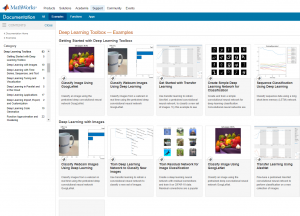
Deep Network Designer (DND) has been Deep Learning Toolbox’s flagship app since 2018. Last release (20a) introduced training inside the app, but you could only train for image classification. In 20b training is massively expanded to cover many more deep learning applications.
The new feature allows for importing and visualization new datatypes, which enables workflows such as time-series, image-to-image regression, and semantic segmentation. This example shows how to train a semantic segmentation network using DND.
|
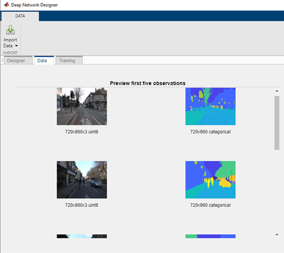
Deep Network Designer visualization of input data
|
Give us the highlights: There is much more flexibility in the app this release; you can import any datastore and train any network that works with trainnetwork. This opens up timeseries training and image-to-image regression workflows. You can also visualize the input data directly in the app prior to training. Although this is a simple example, it walks through each of these steps and trains semi-quickly.
Any challenges when creating the example? Not challenges per se, but this example touches on a lot of components: semantic segmentation, image processing, computer vision, and how to use and explain it all within the context of the app. Also, the algorithm uses unetlayers so I got to read up on that too.
What else?
- I also created a “concept page” which was a result of trying and testing the app. I wanted to offer data that you can immediately use with the app. A lot of other examples require cleaning and preprocessing, so instead, I wanted to deliver out-of-the-box data that you can just run. If you start with blank MATLAB you can run any of these code snippets (time series, image, pixels etc), which can be used as a starting point for the DND workflow. This is the code for quickly importing the digits data:
dataFolder = fullfile(toolboxdir('nnet'),'nndemos','nndatasets','DigitDataset');

imds = imageDatastore(dataFolder, 'IncludeSubfolders',true, ...
    'LabelSource','foldernames');

imageAugmenter = imageDataAugmenter( 'RandRotation',[1,2]);
augimds = augmentedImageDatastore([28 28],imds,'DataAugmentation',imageAugmenter);

augimds = shuffle(augimds);
Use these code snippets as a starting point and try adapting them for your own data set and application!
- There’s also an image-to-image regression example I created for those interested in a semantic segmentation alternative. This example also walks through using DND for the complete workflow using image deblurring.
Besides your work, any recommendations for other examples to try in 20b?
- LIME is pretty cool: it’s interesting (and useful) to see what a network has actually learned (we cover that in the next featured example below!)
- There’s a new style transfer example available on github too!
Thanks to Jess for the insight and recommendations! The example is here.
Visualize predictions with imageLIME
Grad-CAM and occlusion sensitivity have been used in Deep Learning Toolbox for a release or two to visualize the areas of the data that make the network predict a specific class. This release features a new visualization technique called LIME. This new example uses imageLIME for visualizations.
What is LIME - in 60 seconds or less? LIME stands for local interpretable model-agnostic explanation, and it’s slightly more complicated than the Grad-CAM algorithm to implement. You provide a single data point to the LIME algorithm, and the algorithm perturbs the data to generate a bunch of sample data. The algorithm then uses those samples to fit a simple regression model that has the same classification behavior as the deep network. Because of the perturbations, you can see which parts of the data are most important for the class prediction. Model-agnostic means it doesn’t matter how you got your original model, it’s simply showing scores localized to the changes of the initial piece of data.
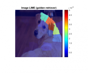
The main thing to keep in mind is LIME computes maps of the feature importance to show you the areas of the image that have the most influence on the class score. These regions are essential for that particular class prediction, because if they are removed in the perturbed images the score goes down.
As an aside I have to ask: What’s with the image of the dog? We use it a lot for deep learning: it ships with MATLAB and it’s nice to show! The dog’s name is Sherlock and she belongs to a developer at MathWorks. We decided to use this image for the example because we use the same image with occlusion sensitivity and grad-CAM. Using the same image for all visualizations can help you compare and highlight the similarities or differences between the algorithms. In fact, in the example we compare LIME with Grad-CAM.
You can visualize all 3 algorithms side-by-side below:
Showing side-by-side comparison of visualization algorithms available. All algorithms can show heat maps, but LIME can also show the nice superpixel regions (as seen above).
LIME results can also be plotted by showing only the most important few features:

Any challenges when creating the example? This example is a nice continuation from the other visualization work that came before, so it was fairly straightforward to create this example. The only challenge was deciding on the name of the function: Should we call it imageLIME, or just LIME, or even deepLIME. We debated this for a while.
What else?
- As the name implies, the function imageLIME is used primarily for images. However, it works with any network that uses an imageInputLayer, so it can work with time-series, spectral or even text data.
- Here’s a really fun example my colleague used as an augmentation of this example. She showed the algorithm a picture of many zoo animals, and then used LIME to home in on a particular animal.
This example makes LIME work almost like a semantic segmentation network for animal detection!
net = googlenet;
inputSize = net.Layers(1).InputSize(1:2);
img = imread("animals.jpg");

img = imresize(img,inputSize);
imshow(img)

classList = [categorical("tiger") categorical ("lion") categorical("leopard")];
[map,featMap,featImp] = imageLIME(net,img,classList);
fullMask = zeros(inputSize);

for j = 1:numel(classList)
  [~,idx] = max(featImp(:,j));
  mask = ismember(featMap,idx);
  fullMask = fullMask + mask;
end

maskedImg = uint8(fullMask).*img;
imshow(maskedImg)
Besides this example, any other examples you like for 20b?
- minibatchqueue is new. It’s not super flashy but it’s very useful. Minibatchqueue is a new way to manage and process data for the custom training workflow. It’s just a nicer way of managing data for custom training loops and much cleaner to read.
Thanks to Sophia for the info and recommendations, especially the animal images!! The example is here.
New Feature Input for trainnetwork
Our final featured example today highlights a more advanced example. Prior to this release, network support was limited to image or sequence data. 20b introduced a new input layer: featureInputLayer.
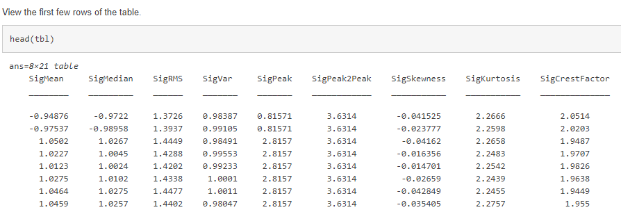
This layer unlocks new type of data: generic data. It’s no longer a requirement to be continuous data, such as time-series data. The data featured in this example is gear shift data, so each column corresponds to one value from a sensor: such as temperature and other single values. Each row is an observation.
 Link to example is here.
This workflow sounds like a traditional machine learning workflow. Any concerns about overlap? This example closes the gap between traditional machine learning and allows the user to explore both ML and DL. Prior to this release, individual feature data could only work in a traditional machine learning workflow.
Do you expect that feature inputs to run faster than other deep learning examples? Of course, I have to say, “it depends,” but I’ve found this example trains very fast (a few seconds). You’re not dealing with large images, so it could train faster. Also, if your model is simpler as this one is, you may need less time as well.
Any challenges when creating the example? After you get the data in, it’s basically the same workflow as training any network, but keep in mind two things when going through this workflow:
Link to example is here.
This workflow sounds like a traditional machine learning workflow. Any concerns about overlap? This example closes the gap between traditional machine learning and allows the user to explore both ML and DL. Prior to this release, individual feature data could only work in a traditional machine learning workflow.
Do you expect that feature inputs to run faster than other deep learning examples? Of course, I have to say, “it depends,” but I’ve found this example trains very fast (a few seconds). You’re not dealing with large images, so it could train faster. Also, if your model is simpler as this one is, you may need less time as well.
Any challenges when creating the example? After you get the data in, it’s basically the same workflow as training any network, but keep in mind two things when going through this workflow:
- You can’t do image-based convolutions, but with data like this the network may not need to be as complex.
- Another thing to consider is categorical data. Sensor data can sometimes be a string value, such as “on” or “off” rather than a numeric value. Deep learning networks won’t accept these values as input, so you have to use onehotencode (also a new function that makes this workflow possible) which will convert the categorical labels to binary.
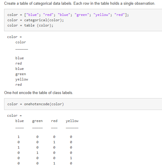 Showing easy implementation of onehotencode
- Another extension of this example is using both image and feature data in the same network. This example uses handwritten digits (images), and the angle (features) as input. It uses a custom training loop to handle the different inputs, but it unlocks a brand-new network type.
Besides this example, any other examples you like for 20b?
- If you’re doing seriously low-level stuff, you’ll be using the model function option to define and train your network. This concept page shows all built-in layers, the default initializations, and how implement it yourself.
- There’s also a new flowchart page which shows which method of training will be best for your particular deep learning problem. This will help you decide between the simpler trainnetwork option, to the more advanced custom training loop options.
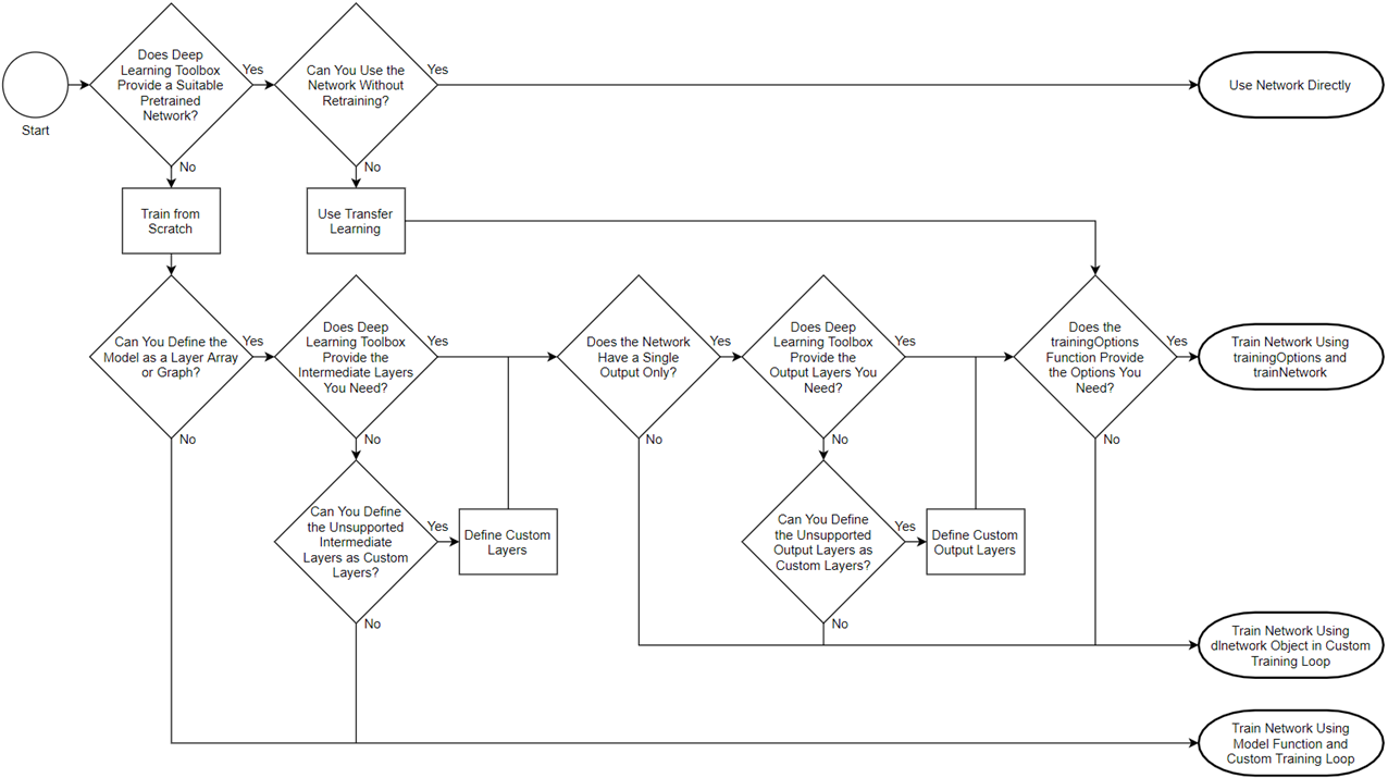 Flowchart helping determine which training style to use. Link to the full flowchart example is here.
Thanks to Ieuan for the info and recommendations! Link to the example is here.
Straight from the doc team to you! I have to say I’m a fan of the “concept pages” and hope that trend continues! Thanks again to Jess, Sophia, and Ieuan. I hope you found this informative and helpful. If you have any questions for the team, leave a comment below!
Flowchart helping determine which training style to use. Link to the full flowchart example is here.
Thanks to Ieuan for the info and recommendations! Link to the example is here.
Straight from the doc team to you! I have to say I’m a fan of the “concept pages” and hope that trend continues! Thanks again to Jess, Sophia, and Ieuan. I hope you found this informative and helpful. If you have any questions for the team, leave a comment below!


评论
要发表评论,请点击 此处 登录到您的 MathWorks 帐户或创建一个新帐户。