
Deep Wine Designer
This post is another from Ieuan Evans, who brought us Deep Beer Designer, back today to talk about wine! It's a longer post than usual, but packed with useful information for Deep Learning for Text. If you're looking for a unique text example, this is for you!
Following my last blog post about how to use MATLAB to choose the perfect beer, I decided to explore what I could do with deep learning and wine.
Similar to beer, the number of different choices of wine is overwhelming. Before I can select a wine, I need to work out what grape varieties of wine I actually like.
Could MATLAB help me with this? If I describe my
perfect wine to MATLAB, will it be able to select one for me? Which characteristics of different wine varieties stand out?
There are two common approaches to a text classification problem like this:
word = "France"
 The resulting image is not particularly exciting. It is a C-by-S array, where C is the number of features of the word embedding (the embedding
dimension) and S is the number of words in the text (the sequence length). When formatted as 1-by-N hyperspectral image with C channels, you can
input this data to a CNN and apply sliding filters of height 1. These are known as 1-D convolutions.
The resulting image is not particularly exciting. It is a C-by-S array, where C is the number of features of the word embedding (the embedding
dimension) and S is the number of words in the text (the sequence length). When formatted as 1-by-N hyperspectral image with C channels, you can
input this data to a CNN and apply sliding filters of height 1. These are known as 1-D convolutions.
 To quickly verify whether text classification might be possible, let's quickly create word clouds for a selection of classes and inspect the differences between them. If you have Text Analytics Toolbox installed, then the wordcloud function automatically preprocesses string input. For better visualizations, let's also remove a list of common words and the grape varieties from the text.
 The word clouds show that the distributions of words amongst each grape variety are different. Even though words like "fruit" and "berry" appear to commonly describe some of these varieties, the word clouds show that the distributions of words among each grape variety are different.
This shows that there are grounds to train a classifier on the text data. Excellent!
The word clouds show that the distributions of words amongst each grape variety are different. Even though words like "fruit" and "berry" appear to commonly describe some of these varieties, the word clouds show that the distributions of words among each grape variety are different.
This shows that there are grounds to train a classifier on the text data. Excellent!
Bring in the description and variety fields from the table.
 Most of the reviews contain 80 or fewer words. Let's use this as our sequence length by specifying 80 in our custom transform function. The transformTextData function, takes the data read from a tabularTextDatastore object and returns a table of predictors and responses.
 For validation, let's also create a transformed datastore containing the validation data using the same steps.
 Here we can see that the training accuracy converges to about 93% and the validation accuracy converges to about 63%. This suggests that the
network might be overfitting to the training data. In particular, it might be learning characteristics of the training data that does not generalize well to the
validation data. More investigation is needed here!
Here we can see that the training accuracy converges to about 93% and the validation accuracy converges to about 63%. This suggests that the
network might be overfitting to the training data. In particular, it might be learning characteristics of the training data that does not generalize well to the
validation data. More investigation is needed here!
 Here, the network has classified four out of eight correctly. Though I'm tempted to let it get away with saying Cava is a sparkling blend (technically, the network is correct). Similarly, saying Syrah instead of Shiraz is forgivable since they are the same variety under different names.
So let's say 6 out of 8... Great!
Here, the network has classified four out of eight correctly. Though I'm tempted to let it get away with saying Cava is a sparkling blend (technically, the network is correct). Similarly, saying Syrah instead of Shiraz is forgivable since they are the same variety under different names.
So let's say 6 out of 8... Great!
 Here, we can see that the network has learned that the phrases "Rich and slightly sweet" and "notes of lychee" is a strong indication of the Gewürztraminer variety, and similarly, the phrases "straw colored" and "Notes of peaches" are less characteristic for this variety.
Now, let's visualize one of the misclassified varieties using the same technique.
Here, we can see that the network has learned that the phrases "Rich and slightly sweet" and "notes of lychee" is a strong indication of the Gewürztraminer variety, and similarly, the phrases "straw colored" and "Notes of peaches" are less characteristic for this variety.
Now, let's visualize one of the misclassified varieties using the same technique.
 Here, we can see that the network understands many of the phrases as strong indications of the Merlot variety with the exception of "high alcohol content". Similarly, the second plot shows that the network understands only some of the phrases in the text as being characteristic of the Zinfandel variety, however, the phrase "strong tannins" and phrases containing "cherry" or "cherries" are particularly uncharacteristic in comparison.
Perfect! Now I can get MATLAB to help me identify the wines I like. Furthermore, I can visualize the predictions made by the network and perhaps learn a few more things myself. I think I better test this network at a few more wine tastings...
All helper functions can be found using the Get the MATLAB Code link below.
Thanks to Ieuan for this very informative and wine-filled post. He originally wanted to title this post, "Grapes of Math" but I've implemented no-pun policy on the blog. I especially like that he field tests his code by going to wine tastings, now that's dedication! Have a question for Ieuan? Leave a comment below.
Here, we can see that the network understands many of the phrases as strong indications of the Merlot variety with the exception of "high alcohol content". Similarly, the second plot shows that the network understands only some of the phrases in the text as being characteristic of the Zinfandel variety, however, the phrase "strong tannins" and phrases containing "cherry" or "cherries" are particularly uncharacteristic in comparison.
Perfect! Now I can get MATLAB to help me identify the wines I like. Furthermore, I can visualize the predictions made by the network and perhaps learn a few more things myself. I think I better test this network at a few more wine tastings...
All helper functions can be found using the Get the MATLAB Code link below.
Thanks to Ieuan for this very informative and wine-filled post. He originally wanted to title this post, "Grapes of Math" but I've implemented no-pun policy on the blog. I especially like that he field tests his code by going to wine tastings, now that's dedication! Have a question for Ieuan? Leave a comment below.

- Train a long short-term memory (LSTM) network that treats text data as a time series and learns long-term dependencies between time steps.
- Train a convolutional neural network (CNN) that treats text data as hyperspectral images and learns localized features by applying sliding convolutional filters.
Background: Word Embeddings
To convert text to hyperspectral images, we can use a word embedding that maps a sequence of words to a 2-D array representing an image. In other words, a word embedding maps words to high-dimensional vectors. These vectors sometimes have interesting properties. For example, given the word vectors corresponding to Italy, Rome, Paris, and France you might discover the relationship:Italy – Rome + Paris ≈ France
That is, the vector corresponding to the word Italy without the components of the word Rome but with the added components of the word Paris is approximately equal to the vector corresponding to France. To do this in MATLAB, we can use the Text Analytics Toolbox™ Model for fastText English 16 Billion Token Word Embedding support package. This word embedding maps approximately 1,000,000 English words to 1-by-300 vectors. Let's load the word embedding using the fastTextWordEmbedding function.emb = fastTextWordEmbedding;Let's visualize the word vectors Italy, Rome, Paris, and France. By calculating the word vectors using the word2vec function, we can see the relationship:
italy = word2vec(emb,"Italy");
rome = word2vec(emb,"Rome");
paris = word2vec(emb,"Paris");

word = vec2word(emb,italy - rome + paris)
Words to Images
To use a word embedding to map a sequence of words to an image, let's split the text into words using tokenizedDocument and convert the words to a sequence vectors using doc2sequence.str = "The rain in Spain falls mainly on the plain."; document = tokenizedDocument(str); sequence = doc2sequence(emb,document);Let's view the hyperspectral images corresponding to this sequence of words.
figure
I = sequence{1};
imagesc(I,[-1 1])
colorbar
xlabel("Word Index")
ylabel("Embedding Feature")
title("Word Vectors")
The resulting image is not particularly exciting. It is a C-by-S array, where C is the number of features of the word embedding (the embedding
dimension) and S is the number of words in the text (the sequence length). When formatted as 1-by-N hyperspectral image with C channels, you can
input this data to a CNN and apply sliding filters of height 1. These are known as 1-D convolutions.
Load Wine Reviews Data
Let's download the Wine Reviews data from Kaggle and extract the data into a folder named wine-reviews. After downloading the data, we can read the data from winemag-data-130k-v2.csv into a table using the readtable function. The data contains special characters such as the é in Rosé, so we must specify the text encoding option too.filename = fullfile("wine-reviews","winemag-data-130k-v2.csv");
data = readtable(filename,"Encoding","UTF-8");
data.variety = categorical(data.variety);
Explore Wine Reviews Data
To get a feel for the data, let's visualize the text data using word clouds. First create a word cloud of the different grape varieties.figure;
wordcloud(data.variety);
title("Grape Varieties")
To quickly verify whether text classification might be possible, let's quickly create word clouds for a selection of classes and inspect the differences between them. If you have Text Analytics Toolbox installed, then the wordcloud function automatically preprocesses string input. For better visualizations, let's also remove a list of common words and the grape varieties from the text.
labels = ["Gewürztraminer" "Chardonnay" "Nebbiolo" "Malbec"];
commonWords = ["wine" "Drink" "drink" "flavors" "finish" "palate" "notes" "aromas"];

figure
for i = 1:4
  subplot(2,2,i)
  label = labels(i);
  idx = data.variety == label;

  str = data.description(idx);
  documents = tokenizedDocument(str)
  documents = removeWords(documents,commonWords);
  documents = removeWords(documents,labels);
  str = joinWords(documents);

  wordcloud(str);
  title(label)
end
The word clouds show that the distributions of words amongst each grape variety are different. Even though words like "fruit" and "berry" appear to commonly describe some of these varieties, the word clouds show that the distributions of words among each grape variety are different.
This shows that there are grounds to train a classifier on the text data. Excellent!

Prepare Text Data for Deep Learning
To classify text data using convolutions, we need to convert the text data into images. To do this, let's pad or truncate the observations to have a constant length S and convert the documents into sequences of word vectors of length C using the pretrained word embedding. We can then represent a document as a 1-by-S-by-C image (an image with height 1, width S, and C channels). To convert text data from a CSV file to images, I have a helper function at the end of this post called transformTextData. It creates a tabularTextDatastore object and uses the transform function with a custom transformation function that converts the data read from the tabularTextDatastore object to images for deep learning. In this example, we'll train a network with 1-D convolutional filters of varying widths. The width of each filter corresponds the number of words the filter can see (the n-gram length). The network has multiple branches of convolutional layers, so it can use different n-gram lengths.Clean up Data
Remove reviews without a label.idxMissing = ismissing(data.variety); data(idxMissing,:) = [];Remove any reviews where the grape variety is not one of the top 200 varieties in the data. (If you can't find a wine you like in the top 200 choices available, MATLAB probably can't help you.)
numClasses = 200;
[classCounts,classNames] = histcounts(data.variety);

[~,idx] = maxk(classCounts,numClasses);
classNames = classNames(idx);

idx = ismember(data.variety,classNames);
data = data(idx,:);
Remove the unused categories from the data.
data.variety = removecats(data.variety);
classNames = categories(data.variety);
Partition Data
To help evaluate the performance of the network, let's partition the data into training, testing, and validation sets. Let's set aside 30% of the data for validation and testing (two partitions of 15%).cvp = cvpartition(data.variety,'HoldOut',0.3);
filenameTrain = fullfile("wine-reviews","wineReviews_" + numClasses + "_classes_Train.csv");
dataTrain = data(training(cvp),:);
writetable(dataTrain,filenameTrain,"Encoding","UTF-8");
dataHeldOut = data(test(cvp),:);
cvp = cvpartition(dataHeldOut.variety,'HoldOut',0.5);
filenameValidation = fullfile("wine-reviews","wineReviews_" + numClasses + "_classes_Validation.csv");
dataValidation = dataHeldOut(training(cvp),:);
writetable(dataValidation,filenameValidation,"Encoding","UTF-8");
filenameTest = fullfile("wine-reviews","wineReviews_" + numClasses + "_classes_Test.csv");
dataTest = dataHeldOut(test(cvp),:);
writetable(dataTest,filenameTest,"Encoding","UTF-8"); |
 Need a break from reading code? Read how researchers are using MATLAB for making better beer and wine in this article.
 |
miniBatchSize = 128;
ttdsTrain = tabularTextDatastore(filenameTrain, ...
'SelectedVariableNames',["description" "variety"], ...
'ReadSize',miniBatchSize);
Specify Input Size
To input the text data into the network, we need to convert the text to images with a fixed size by padding or truncating the sequences. Ideally, we need to choose a value that minimizes both the amount of padding added to the sequences and the amount of data discarded due to truncation. Let's try to approximate the number of words in each review by counting the number of spaces and plotting the sequence lengths in a histogram.
Most of the reviews contain 80 or fewer words. Let's use this as our sequence length by specifying 80 in our custom transform function. The transformTextData function, takes the data read from a tabularTextDatastore object and returns a table of predictors and responses.
sequenceLength = 80;
tdsTrain = transform(ttdsTrain, @(data) transformTextData(data,sequenceLength,emb,classNames));
The predictors are 1-by-S-by-C arrays, where S is the sequence length and C is the number of features. The responses are the categorical labels.
preview(tdsTrain)
For validation, let's also create a transformed datastore containing the validation data using the same steps.
ttdsValidation = tabularTextDatastore(filenameValidation, ...
    'SelectedVariableNames',["description" "variety"], ...
    'ReadSize',miniBatchSize);
tdsValidation = transform(ttdsValidation, @(data) transformTextData(data,sequenceLength,emb,classNames))
Define Network Architecture
Let's now define the network architecture for the classification task, we can use deepNetworkDesigner to create the network. |
The following describes the network architecture:
|
Specify Training Options
numIterationsPerEpoch = floor(numObservationsTrain/miniBatchSize);
options = trainingOptions('adam', ...
'MaxEpochs',50, ...
'Shuffle','never', ...
'MiniBatchSize',miniBatchSize, ...
'ValidationData',tdsValidation, ...
'ValidationFrequency',numIterationsPerEpoch, ...
'Plots','training-progress', ...
'Verbose',false);
Train Network
Finally, we can train the network! Let's train the network using the trainNetwork function. Depending on your hardware, this can take a long time. If you are having trouble with hardware or training, you can email Johanna for a copy of the trained network.caberNet = trainNetwork(tdsTrain,lgraph,options);
save("caberNet.mat","caberNet")
*Note from Johanna to Ieuan: I have a no-pun policy on this blog, and "caberNet" is borderline, so consider this a warning.
Here we can see that the training accuracy converges to about 93% and the validation accuracy converges to about 63%. This suggests that the
network might be overfitting to the training data. In particular, it might be learning characteristics of the training data that does not generalize well to the
validation data. More investigation is needed here!
Test Network
Now the network is trained, we can test it using the held-out test data. First, let's create a transformed datastore containing the held-out test data.ttdsTest = tabularTextDatastore(filenameTest, ...
'SelectedVariableNames',["description" "variety"], ...
'ReadSize',miniBatchSize);
tdsTest = transform(ttdsTest, @(data) transformTextData(data,sequenceLength,emb,classNames));
tbl = readall(ttdsTest);
labelsTest = tbl.variety;
YTest = categorical(labelsTest,classNames);
YPred = classify(caberNet,tdsTest,'MiniBatchSize',miniBatchSize);
accuracy = 0.6397
Here, we can see that the network is about 64% accurate on the held-out test data. Given the varied and subjective nature of wine tasting notes, I think this is a good score!
Make Predictions on New Data
The next step is to try out the classifier in the real world! Here are some notes from a recent wine tasting I attended.- “A crisp, golden coloured, bubbly wine. On the nose, there are aromas of citrus fruits alongside ripe stone fruits. On the palete, vibrant notes of apple and creamy textures.”
- “Straw coloured with a slight hint of green. Notes of peaches and nectarines. Rich and slightly sweet, intense notes of lychee. Strong minerality with some sweetness.”
- “Pale straw in colour with zesty citrus fruit on the nose. On the palate, intense gooseberry and crisp lime flavours with slight hints of oak.”
- “Deep golden colour. Strong aromas of toast and butter with strong hints of oak. On the palate, intense flavours of ripe banana and cooked apples.”
- “Very light bodied wine and pale in colour. Aromas of strawberries and forest fruits. Slightly oaked with slight tannins. Vibrant taste of red cherries.”
- “Medium bodied and brick-red in colour. On the nose, black cherry, and violet. Complex flavours including strong tannins coupled with flavours of black fruits and pepper.”
- “Deep ruby red in colour. Aromas of dark cherries, oak, and clove. Slightly smokey in taste with strong hints of blackberries and licorce.”
- “Strong aromas of blackcurrent and blueberries. A very big wine with high alcohol content. Intense flavour on the palate with a long finish. Vibrant flavors of black fruits and spices.”
sequencesNew = text2sequence(emb,str,sequenceLength);
[YNewPred,scoresNew] = classify(caberNet,sequencesNew);

tbl = table;
tbl.PredictedVariety = YNewPred;
tbl.TrueVariety = YNewTest
Here, the network has classified four out of eight correctly. Though I'm tempted to let it get away with saying Cava is a sparkling blend (technically, the network is correct). Similarly, saying Syrah instead of Shiraz is forgivable since they are the same variety under different names.
So let's say 6 out of 8... Great!
Visualize Network Predictions
For image classification problems, you can visualize the predictions of a network by taking an image, deleting a patch of the image, measure if the classification gets better or worse, then overlay the results on the image. In other words, if you delete a patch of the image and the classification gets worse, then that patch must contain features pertaining to the true class. Similarly, if you delete a patch of the image, and the classification gets better, then that patch must contain features pertaining to a different class and thus confuses the classifier. We can do this using the occlusionSensitivity function. Let's select one of the observations of the text data where the network has predicted the correct label.idxObservation = 2; strNew = str(idxObservation) labelTest = YNewTest(idxObservation)strNew = "Slightly straw colored with a hint of greenness. Notes of peaches and nectarines. Rich and slightly sweet, intense notes of lychee. A soft finish with some sweetness." labelTest = "Gewürztraminer" Let's view the occlusion sensitivity scores using the function plotOcclusion, which I have listed at the end of the blog post. This shows which patches of words contribute most to the prediction.
h = figure;
h.Position(3) = 1.5 * h.Position(3);
plotOcclusion(caberNet,emb,strNew,sequenceLength,labelTest)
Here, we can see that the network has learned that the phrases "Rich and slightly sweet" and "notes of lychee" is a strong indication of the Gewürztraminer variety, and similarly, the phrases "straw colored" and "Notes of peaches" are less characteristic for this variety.
Now, let's visualize one of the misclassified varieties using the same technique.
idxObservation = 8;
strNew = str(idxObservation)

labelTest = YNewTest(idxObservation)
strNew = "Strong aromas of black cherry. Powerful taste with a high alcohol content. Rich flavor with strong tannins and a long finish. Vibrant flavors of cherries and a hint of pepper." labelTest = "Zinfandel"
h = figure;
h.Position(3) = 1.5 * h.Position(3);
h.Position(4) = 1.5 * h.Position(4);
plotOcclusion(caberNet,emb,strNew,sequenceLength,labelTest)
Here, we can see that the network understands many of the phrases as strong indications of the Merlot variety with the exception of "high alcohol content". Similarly, the second plot shows that the network understands only some of the phrases in the text as being characteristic of the Zinfandel variety, however, the phrase "strong tannins" and phrases containing "cherry" or "cherries" are particularly uncharacteristic in comparison.
Perfect! Now I can get MATLAB to help me identify the wines I like. Furthermore, I can visualize the predictions made by the network and perhaps learn a few more things myself. I think I better test this network at a few more wine tastings...
All helper functions can be found using the Get the MATLAB Code link below.
Thanks to Ieuan for this very informative and wine-filled post. He originally wanted to title this post, "Grapes of Math" but I've implemented no-pun policy on the blog. I especially like that he field tests his code by going to wine tastings, now that's dedication! Have a question for Ieuan? Leave a comment below.
Copyright 2018 The MathWorks, Inc. Get the MATLAB code
- Category:
- Deep Learning


See Also
-

Deep Beer Designer
Blogs


Comments
To leave a comment, please click here to sign in to your MathWorks Account or create a new one.