 Cleve’s Corner: Cleve Moler on Mathematics and Computing
 The MATLAB Blog
 Guy on Simulink
 MATLAB Community
 Artificial Intelligence
 Developer Zone
 Stuart’s MATLAB Videos
 Behind the Headlines
 File Exchange Pick of the Week
 Hans on IoT
 Student Lounge
 MATLAB ユーザーコミュニティー
 Startups, Accelerators, & Entrepreneurs
 Autonomous Systems
 Quantitative Finance
 MATLAB Graphics and App Building
Managing and Fine-Tuning Portfolio Optimization Workflows with Experiment Manager
The following blog was written by Sara Galante, Senior Finance Application Engineer at Mathworks.
The code used to develop this example can be found on GitHub here: Managing Asset Allocation with the Experiment Manager
Portfolio optimization, a complex task in finance, becomes increasingly challenging when we want to fine-tune multiple parameters simultaneously – particularly when trying to balance returns, risks, and other outputs. With the aid of MathWorks’ Experiment Manager App, this intricate process becomes remarkably more manageable and efficient. By leveraging the Experiment Manager’s capabilities, researchers and practitioners gain a powerful tool to systematically explore and fine-tune parameters in portfolio optimization. In this blog post, we will delve into the utilization of the Experiment Manager App, focusing on its ability to navigate the complexities of multi-variable optimization. Through the development of a practical example, we will highlight how the Experiment Manager App simplifies the fine-tuning of objective functions and penalty parameters, ultimately leading to more robust and optimized portfolio allocations.
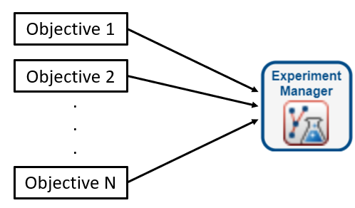
Experiment Manager enables users to fine tune and manage multiple portfolio objectives in one place
The content of this blog was also presented as a talk! View the video here:

Overview of the Experiment Manager App:
The Experiment Manager App is a powerful tool provided in MATLAB that simplifies the process of designing, executing, and managing experiments. It offers a user-friendly interface that allows researchers and practitioners to explore different combinations of parameters and efficiently analyze the results. Let’s delve deeper into the key features and benefits of the Experiment Manager App.
- Experiment Design: The Experiment Manager App provides a convenient interface to design and execute experiments. We can see this by looking at Figure 1 below.

Figure 1.
Users can begin by specifying the variables they wish to test in the “Hyperparameters” section. For this example, our hyperparameters are the optimization objective function, or “Technique”, and the penalty parameter, denoted as “lambda.” Ranges for each of these variables can be specified directly as well, allowing the user to fine tune as needed. Additionally, the user must indicate exactly how the experiment must be executed by writing and specifying a “Training Function.” We can think of this as a blueprint for setting up the experiments, shown by Figure 2.
Figure 2.
The training function for our example defines what routine each experiment should follow, including loading the data, initializing our portfolio object, and specifying which metrics the app should capture in line 2. The hyperparameters are identified in the code through the “params” variable, shown in lines 11 and 18 in Figure 3.
Figure 3. - Automated Execution:Once the experiment is designed, the Experiment Manager App automates the execution process. It systematically sweeps through each combination of hyperparameters, eliminating the need for manual iteration. This automation saves significant time and effort, especially when dealing with a large number of parameters or numerous iterations.
- Data Collection and Organization:The Experiment Manager App collects and organizes the results of each experiment iteration. It records the performance metrics, optimization outputs, and any other relevant data in an organized table, shown in Figure 4.

Figure 4.This organization simplifies the analysis phase and allows for easy comparison and interpretation of the results.
- Efficient Parameter Sweeping: The Experiment Manager App excels in parameter sweeping tasks, where multiple parameters are simultaneously varied to explore their combined effects. It efficiently sweeps through the defined ranges of variables, executing the optimization algorithm for each combination. This capability is particularly useful in portfolio optimization, where multiple variables need to be fine-tuned simultaneously.
- Parallel Computing Support:To expedite the execution of experiments, the Experiment Manager App supports parallel computing. It can leverage the computational power of multicore processors or clusters to execute multiple iterations simultaneously. This parallelization significantly reduces the overall execution time, making it an ideal choice for computationally intensive tasks. The parallel computing functionality isn’t explored in this example, but can be useful for computationally heavy tasks.
By leveraging the Experiment Manager App, researchers and practitioners can streamline their experimentation process, automate repetitive tasks, and gain valuable insights into the impact of different variables on their optimization models and the interaction of said variables with each other. It empowers users to make informed decisions, optimize their models efficiently, and ultimately achieve their desired outcomes.
Developing the Example:
To provide a more detailed understanding of how the Experiment Manager App can be utilized for fine-tuning variables in portfolio optimization, let’s delve into the step-by-step process of developing the example.
- Importing Financial Data:In Figure 2, we begin by importing the financial data into MATLAB. This data includes simulated pricing data, created using geometric Brownian motion, and consists of 39 simulated stocks. MATLAB provides various functions and tools to facilitate data import and helps to preprocess a wide variety of data formats, ensuring that the data is in a suitable format for analysis.
- Defining Constraints:Once the data is imported, we define the constraints for the portfolio optimization problem. These constraints may include budget constraints, asset allocation limits, and any other specific requirements based on your investment strategy. MATLAB provides a portfolio framework via the Portfolio object that allows for the incorporation of constraints into a portfolio optimization model with ease.
- Objective Function Selection:In Figure 3, we utilize the Experiment Manager App to choose through the different objective functions via case statements. Objective functions define the criteria by which the optimization algorithm evaluates and selects the optimal allocation. For this example, we look at equal weighting, most-diversified portfolio, and equal risk contribution objective strategies using the Portfolio object’s built-in custom objective functionality. By trying these objective functions, you can observe the impact on the optimized portfolios.
- Penalty Parameter Selection:In addition trying different objective functions, we use the Experiment Manager App to iterate through a range of penalty parameters. The penalty parameter controls the level of risk aversion and helps balance the trade-off between the different objectives and the portfolio risk. By systematically varying the penalty parameter, you can assess its impact on the optimized portfolios and identify the optimal level of risk aversion.
- Running the Portfolio Optimization Scenarios:For each experiment, run the portfolio optimization algorithm using the selected objective function and penalty parameter. The Financial Toolbox provides the Portfolio object with functionality that can be used to solve custom objective problems. Evaluate the resulting portfolios based on performance metrics such as expected returns, volatility, and turnover measures.
- Recording Results:Record the performance metrics and optimization outputs for each. The Experiment Manager App automatically collects and organizes this data, as seen in Figure 4, making it easy to analyze and compare the results later. This organized data allows for efficient post-processing and identification of trends or patterns across different combinations of objective functions and penalty parameters.
- Visualizing and Analyzing Results:Utilize the visualization and analysis tools provided by the Experiment Manager App to gain insights from the recorded results. Generate plots, charts, and statistical summaries to visualize the performance of different portfolios. This analysis enables the identification of optimal combinations of objective functions and penalty parameters that align with your investment goals and risk tolerance. *output to table and use ML program to plot and analyze appropriately*.
By following these steps and leveraging the Experiment Manager App, you can efficiently explore and fine-tune variables in portfolio optimization. The app automates the execution, data collection, and organization processes, saving time and effort. The recorded results and visualizations facilitate a comprehensive analysis of the impact of different variables on the optimized portfolios, enabling you to make informed decisions.
Discussing the Results:
After running the routine, we can examine the results by looking at three bar plots to compare each combination of diversification strategy and penalty parameter.

Returns vs. Penalty Parameter

Volatility vs. Penalty Parameter

Turnover vs. Penalty Parameter
The performance metrics varied when the penalty parameter was modified, with some instances showing significant differences. Upon analyzing the Returns vs Penalty Parameter plot, it becomes evident that increasing the penalty parameter leads to higher returns. Additionally, volatility also rises with an increase in the penalty parameter, while overall turnover decreases. The scenario involving the most diversified portfolio objective presents an intriguing situation. Here, the returns exhibit a substantial increase with the penalty parameter, although the reduction in turnover is not as drastic as observed in the other two objectives being studied.
The decision regarding the selection of Technique and lambda combination for your portfolio can vary depending on the level of risk a portfolio manageris willing to assume in relation to the desired returns. In my opinion, I would advise against opting for the most diversified portfolio since both turnover and volatility are high when using the penalty parameter. However, if the PM is willing to take on slightly more risk in pursuit of higher returns, the equal risk contribution objective is recommended when the penalty parameter is either 3e-6 or 0.01. On the other hand, if the PM is comfortable with slightly lower returns in exchange for reduced risk, the equally weighted scheme is recommended when the penalty parameter is 3e-6 or 0.01.
Conclusion:
In this blog post, we explored how MATLAB’s Experiment Manager App can be utilized to fine-tune parameters in portfolio optimization. By trying different objective function options and penalty parameters, we demonstrated how the Experiment Manager App streamlines the process of exploring different combinations and automating repetitive tasks. Through the analysis of the results, we gain valuable insights into the impact of these variables on the optimized portfolios. The Experiment Manager App proves to be an invaluable tool for researchers and practitioners in the field of finance, enabling them to make informed decisions and optimize their investment strategies efficiently.
The code used to develop this example can be found on GitHub here: Managing Asset Allocation with the Experiment Manager
- Category:
- Asset Management,
- New Features


Comments
To leave a comment, please click here to sign in to your MathWorks Account or create a new one.