The following blog was written by Owen Lloyd , a Penn State graduate who recently join the MathWorks Engineering Development program.

The code used to develop this example can be found on GitHub here.

Background Overview and Motivation

In quantitative finance, the ability to predict future equity prices would be extremely useful for making informed investment decisions. While accurately predicting the daily prices of equities is an extremely difficult problem, deep learning models can serve as one technique for attempting to solve it. Time series prediction with financial data involves forecasting stock prices based on historical data, aiming to capture trends and patterns that can guide trading strategies. The use of deep learning techniques, particularly transformer networks, offers a promising approach for modeling and predicting stock prices. These networks excel at capturing temporal and long-term dependencies within the data, making them well-suited for financial time series analysis.

Throughout this blog post, we will specifically be focusing on transformer deep learning networks. A key advantage of transformer networks is their ability to capture long-range dependencies within data. Compared to an LSTM network, which relies on sequential processing and can struggle to capture long-term dependencies, transformer models utilize self-attention mechanisms to establish connections between all the elements in the sequence, allowing the model to learn relationships and patterns across distant time steps. Another advantage of transformer networks is that they allow for parallel processing and faster training of models with fewer resources, making the network more efficient for modern hardware and larger scale datasets.

For this purpose, a working demo has been developed that provides the workflow for approaching time series prediction for quantitative finance using transformer networks in MATLAB. By leveraging the Deep Learning Toolbox™ and Financial Toolbox™, the demo focuses on predicting the price trends of individual stocks and subsequently backtesting trading strategies based on the predicted time series values. The demo showcases the application of new transformer layers in MATLAB, specifically the positionEmbeddingLayer, selfAttentionLayer, and indexing1dLayer. These layers help to capture and analyze temporal dependencies within financial data. Additionally, the demo covers the process of importing, preprocessing, defining network architecture, training options, hyperparameter tuning, model training, visualization of model performance, and backtesting strategies using the Financial Toolbox™.

Transformer Networks in MATLAB

As previously mentioned, new layers have been introduced in MATLAB R2023a and R2023b that allow for the introduction of transformer layers to network architectures developed using the Deep Network Designer. These new transformer layers are useful for performing time series prediction with financial data due to their ability to capture temporal dependencies and long-term dependencies in the data. The three layers that the following demo utilizes are the positionEmbeddingLayer, selfAttentionLayer, and indexing1dLayer.

• The positionEmbeddingLayer allows for the encoding of the position information of each element within the sequence. By incorporating position embedding, the model can learn to differentiate between different time steps and capture time dependencies within the data.
• The selfAttentionLayer allows the model to weigh the importance of different elements within a sequence. This enables the model to capture the dependencies between all elements in the sequence and learn the relationships between them. Self-attention mechanisms are also effective at capturing long-term dependencies in the data, as they can establish connections between distant time steps, understanding patterns that may have a delayed impact on future outcomes.
• The indexing1dLayer allows for the extraction of data from the specified index of the input data. This enables the network to perform regression on the output of the selfAttentionLayer.

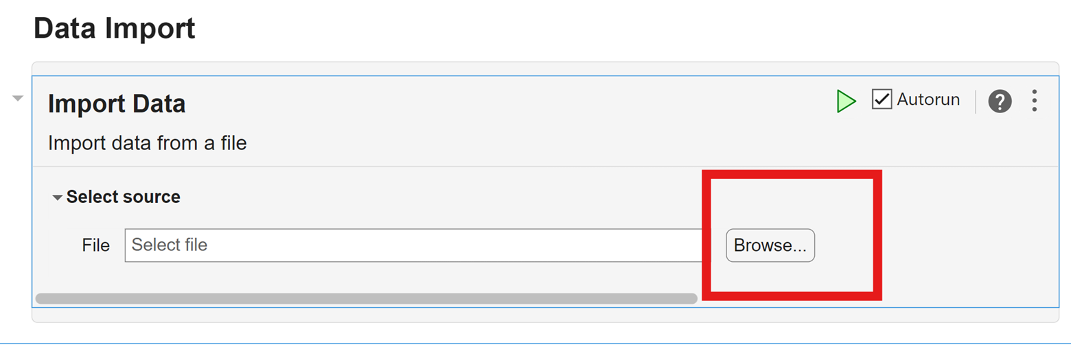
Preprocessing the Data

Figure 1: Average Daily Price of Stocks

Before we can begin training and testing our model, we need to preprocess our data. For this specific demo, we will be predicting the price trends of three individual stocks based on the previous 30 days’ prices.

We begin our preprocessing by partitioning the dataset into training and testing sets, based on the date. For this demo, the cutoff date for the split between training and testing data is the beginning of 2021. After partitioning the dataset, we standardize the training data and normalize the testing data based on the mean and standard deviation of the training data.

With our normalized data, we define a 30-day array of prices corresponding to each price in the dataset to serve as the sequential input for our model. Each 30-day rolling window of actual price data will be used to predict the price on the next day.

Defining the Network Architecture and Training Options

Now that we have preprocessed the data, we can specify our network architecture and training options for our deep learning model. We can specify our network architecture as a series of layers, either using the Deep Network Designer or programmatically in MATLAB. Below is a visualization from the Deep Network Designer of our chosen network architecture.

Figure 2: Transformer Network Architecture

After specifying our network architecture, we also need to specify the training parameters for our model using the trainingOptions function. The training parameters that were used for this demo are solver, MaxEpochs, MiniBatchSize, Shuffle, InitialLearnRate, and GradientThreshold. Within the trainingOptions function, we can specify the execution to use a GPU without needing to change any of our model architecture. To train using a GPU or a parallel pool, the Parallel Computing Toolbox™ is required.

Tuning Hyperparameters

An excellent way to test different hyperparameters for both our network architecture and training options is through the Experiment Manager, which is part of the Deep Learning Toolbox. A tutorial on using the Experiment Manager for training deep learning networks can be found here. Below is the setup and output of an experiment designed to the tune the hyperparameters of the network architecture in this demo.

Figure 3: Hyperparameter Experiment Setup

Figure 4: Hyperparameter Experiment Results

Training the Model and Visualizing Performance

Now that we have defined our network architecture and training options, we can utilize the trainNetwork function to train our model. Below is an image of the training progress partway through the model’s training.

Figure 5: Model Training Progress

With a trained model, we can make predictions on the price of each stock based on the previous 30-day rolling window and compare them to the actual historical stock prices. Below is a plot comparing the model’s predictions to the actual stock prices over the testing data.

Figure 6: Model Prediction Comparison

In addition to visualizing the performance of our model, we can calculate the root mean squared error (RMSE) to get a quantitative estimate of the quality of our predictions. RMSE measures the average difference between the predicted and actual stock prices, providing an indication of the model’s accuracy. The percentage RMSE over the testing data based on the average price of each stock over the testing period is 0.87%, 0.97%, and 1.98% for stocks A, B, and C respectively.

Backtesting Model Predictions on Market Data

While RMSE is a common way to quantify the performance of a set of predictions, our objective with these predictions is to use them to develop a strategy that will be profitable over the testing data. To test the profitability of the trading strategies, we can use the backtesting tools from the Financial Toolbox™. The four trading strategies implemented in this demo are:

• Long Only: Invest all capital across the stocks with a positive predicted return, proportional to the predicted return.
• Long Short: Invest capital across all the stocks, both positive and negative predicted return, proportional to the predicted return.
• Best Bet: Invest all capital into the single asset with the highest predicted return.
• Equal Weight: Rebalance invested capital every day with an equally-weighted allocation between the stocks (benchmark).

Below is an equity curve that shows the performance of each of these trading strategies over the duration of the testing data.

Figure 7: Backtesting Equity Curve

Based on the equity curve above, we can see that our model predictions result in a 24% return when implemented with the Long Only strategy, and a 22% return when implemented with the Best Bet strategy, if we had invested based on them starting in January 2021. The Equal Weight strategy does not consider our model predictions and serves as a baseline performance metric for the underlying equities, with a 13% return over the testing period. These results give an indication that predictions from our model could help develop a profitable trading strategy.

While these backtest results provide insights into the profitability and effectiveness of the trading strategies implemented using the model predictions, the model and the trading strategies used to test its predictive results are not expected to be profitable in a realistic trading scenario. This demo is meant to illustrate a workflow that should be useful with more comprehensive datasets and more sophisticated models and strategies.

Conclusion

In this blog post, we explored how the new transformer layers in MATLAB can be utilized to perform time-series predictions with financial data. We began by preprocessing our data to allow for the application of deep learning tools. We then discussed the implementation of network architectures and training options, as well as the tuning of hyperparameters using the Experiment Manager. After training the model, we evaluated the quality of our predictions through both classic machine learning metrics as well as backtesting on historical data to explore profitability.

The code used to develop this example can be found on GitHub here.