A practical MATLAB walkthrough comparing tracking error and exact exposure approaches.

When you build a factor-based portfolio, the central design choice is how strictly to enforce your factor views. Do you treat target exposures as soft goals or do you impose them as hard constraints that the portfolio must satisfy exactly? That decision can materially change the diversification, concentration, and feasibility of the resulting portfolio.

In this blog post, we use data from the Fama-French Data Library, a widely used academic source, to make the comparison practical in a realistic setting. While the example uses the Fama-French three-factor structure—market (Mkt), size (SMB), and value (HML)—the techniques apply to any multi-factor framework.

We compare two practical optimization approaches using MATLAB®:

1. Tracking Error Minimization—Targets specific factor exposures while allowing small deviations, which can improve diversification and feasibility.
2. Exact Exposure Matching—Enforces target factor exposures exactly using equality constraints, which is useful when strict mandates or regulatory requirements must be met.

1. Load Data and Set Up the Factor Model

We start with one year of price data for the 30 stocks in the Dow Jones Industrial Average® (DJIA), which we convert to returns. Separately, we load the three Fama-French factors: excess market return (Mkt), small minus big (SMB), and high minus low (HML).

After synchronizing the stock and factor data, MATLAB estimates the joint covariance structure using a Portfolio object. In the tracking error formulation, the factor return series are included in that covariance structure even though they are not investable assets. This setup allows the optimization to reflect both stock-return risk and the portfolio’s relationship to the factor returns.

2. Apply Realistic Constraints

Both approaches share the same set of practical constraints:

• Conditional weight bounds: Each stock can either be excluded from the portfolio or, if selected, must hold between 5% and 20%. This keeps positions large enough to matter and small enough to maintain diversification.
• Cardinality limit: The portfolio holds at most 10 stocks. This practical constraint introduces binary asset-selection decisions, making the optimization mixed-integer.
• Full investment: All stock weights sum to 100%, so all capital is invested.
• Factor weights fixed at zero: The factor data series are present in the Portfolio object for covariance estimation, but the optimizer cannot allocate capital to them. Setting their upper and lower bounds to zero enforces this.

3. Approach 1 — Minimize Tracking Error to Factor Targets

This approach finds a portfolio whose factor exposures are close to — but not required to exactly match — a set of predefined targets. In MATLAB, the benchmark is represented by zero weights on all stocks and nonzero weights only on the three factors. The optimization then minimizes tracking error relative to that benchmark.

Target Factor Exposures

• Positive exposure to the overall market (Mkt = 0.013)
• A tilt toward large-cap stocks rather than small-cap stocks (SMB = -0.003)
• A modest tilt toward value over growth (HML = 0.001)

How the Formulation Works

In this formulation, the Fama–French risk factor return series are included in the Portfolio object together with the stock returns, but their weights are fixed at zero. That means the optimizer cannot allocate capital to the factors, even though their return behavior still influences the covariance structure. This lets the tracking error objective guide the portfolio toward the desired factor exposures without introducing a separate factor covariance model.

In the example, MATLAB solves the custom objective with estimateCustomObjectivePortfolio after configuring the mixed-integer solver with setSolverMINLP. The resulting tracking error portfolio uses all 10 available stock slots.

Results

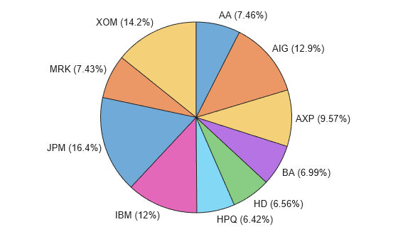
The optimizer selects a diversified set of 10 stocks while satisfying all portfolio constraints.

The resulting portfolio-level exposures are close to the targets, but do not match exactly:

Factor	Target	Achieved
Market	0.0130	0.0116
SMB	-0.0030	-0.0030
HML	0.0010	0.0013

When This Approach Works Well

• You want flexibility around factor targets rather than rigid compliance.
• Diversification and feasibility matter more than exact factor matching.
• You are willing to accept small exposure drift in exchange for a broader, more balanced selection of assets.

4. Approach 2 — Match Factor Exposures Exactly

This approach guarantees that the portfolio’s factor exposures hit the targets precisely. Here, factor data are excluded from the Portfolio object entirely. Instead, MATLAB uses the estimated factor loading matrix Beta to impose equality constraints of the form Beta’ * w = Target Exposure.

The optimization then solves for the minimum-risk portfolio subject to these constraints along with the same weight, cardinality, and budget constraints used in Approach 1.

Results

The resulting portfolio-level exposures match the targets exactly:

Factor	Target	Achieved
Market	0.0130	0.0130
SMB	-0.0030	-0.0030
HML	0.0010	0.0010

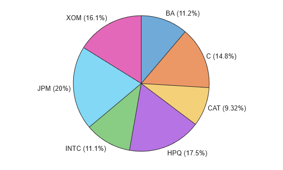
Because the target exposures are enforced directly, the achieved portfolio-level exposures match the targets exactly. The trade-off is reduced freedom for the optimizer, which can lead to fewer holdings, higher concentration, worse risk-return trade-offs, or even infeasibility when the targets are too restrictive.

When This Approach Works Well

• You must meet regulatory or mandate-driven factor targets precisely.
• You need for strict control over portfolio factor exposures.

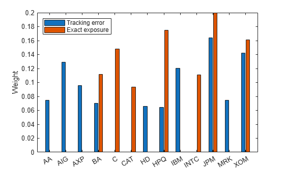
5. Comparing the Two Approaches

A side-by-side view of the asset weights makes the trade-offs concrete.

6. Wrap Up

Choosing between these approaches depends on whether flexibility or precision is the primary objective. Tracking error minimization trades small deviations for better diversification and stronger feasibility under practical constraints. Exact exposure matching guarantees target compliance, but it can do so at the cost of diversification.

Learn More

• Optimize Portfolio Using Fama-French Model — Full example with code, data, and interactive charts
• Portfolio Optimization Using Factor Models — Broader overview of factor-based portfolio optimization in Financial Toolbox™
• Portfolio Optimization with Target Factor Exposures – video