Economists often keep years of work in EViews workfiles: macroeconomic series, model estimates, and curated panel data. The MATLAB Reader for EViews Workfile reads .wf1 and .wf2 files into MATLAB, with no export step or EViews installation. This post shows how to load a workfile, inspect its metadata, plot series, and run a CAPM regression in MATLAB.

Getting Started

Download the reader from the GitHub repository (click the green Code button, then Download ZIP). Unzip it, then add the folder to your MATLAB path:

addpath("MATLAB-Reader-for-EViews-Workfile")

The reader requires MATLAB R2021a or later and no additional toolboxes.

Loading a Workfile

For this walkthrough, we use two publicly available workfiles from the Principles of Econometrics (5th Edition) companion site by Hill, Griffiths, and Lim. The first is Klein’s Model I, a foundational macroeconometric dataset covering US consumption, investment, wages, and output from 1920 to 1941.

Loading it takes one line:

wf = wfread("klein.wf1");

The result is a MATLAB struct. Each field is either a data series or metadata stored in the workfile:

>> fieldnames(wf)
  ans =
      'CN'
      'E'
      'ELAG'
      'G'
      'I'
      'KLAG'
      'P'
      'PLAG'
      'TIME'
      'TX'
      'W'
      'W1'
      'W2'
      'Y'
      'YEAR'
      'Metadata'

Fifteen series: consumption, investment, profits, wages, government spending, capital stock, and more, plus a Metadata field containing the metadata stored in the workfile.

Exploring Metadata

The Metadata struct tells you the workfile’s frequency, time span, and format without opening EViews:

>> wf.Metadata.Frequency
  ans = 1                        % Annual

  >> wf.Metadata.StartYear
  ans = 1920

  >> wf.Metadata.NumObs
  ans = 22

Series Descriptions

EViews workfiles store text descriptions for each variable. The reader preserves them:

>> wf.Metadata.SeriesDescriptions.CN
  ans = '[Display Name] cn  [Description] consumption'

  >> wf.Metadata.SeriesDescriptions.I
  ans = '[Display Name] i  [Description] net investment'

  >> wf.Metadata.SeriesDescriptions.Y
  ans = '[Display Name] y  [Description] total product = cn + i + g - tx'

This embedded documentation means you can identify variables without a separate codebook.

Observed vs. Derived Series

The reader classifies each series as observed (raw data read from the file) or derived (computed from other series by EViews):

>> wf.Metadata.ObservedSeries
  ans =
      "CN"
      "G"
      "I"
      "P"
      "TX"
      "W1"
      "W2"
      "YEAR"

  >> wf.Metadata.DerivedSeries
  ans =
      "E"
      "ELAG"
      "KLAG"
      "PLAG"
      "TIME"
      "W"
      "Y"

For Klein’s model, the observed variables are consumption (CN), government spending (G), net investment (I), profits (P), taxes (TX), and wages in the private and government sectors (W1, W2). The derived variables, total wages (W), total product (Y), lagged values (PLAG, ELAG, KLAG), were computed within EViews.

Accessing Individual Series

Each series is stored as a MATLAB table with observation labels and numeric values:

>> wf.CN
  ans =
       obs       CN
      ______    ____
      "1920"    39.8
      "1921"    41.9
      "1922"      45
      "1923"    49.2
      ...
      "1941"    69.7

Output Format Options

The reader supports four output formats, selectable at load time:

% Timetable — time-indexed, ready for plotting and
  Econometrics Toolbox
  T = wfread("klein.wf1", OutputType="timetable");

  % Table — flat table with all series as columns
  tbl = wfread("klein.wf1", OutputType="table");

  % Matrix — numeric array only (for direct computation)
  M = wfread("klein.wf1", OutputType="matrix");

The timetable output is often the most useful. It works with MATLAB time-series functions, plotting, and toolbox workflows:

>> T = wfread("klein.wf1", OutputType="timetable");
  >> head(T, 4)
       rowTimes       CN      E      ELAG     G      I      KLAG      P     ...
      ___________    ____    ____    ____    ___    ____    _____    ____
      01-Jan-1920    39.8    44.9     NaN    2.4     2.7    180.1    12.7
      01-Jan-1921    41.9    45.6    44.9    3.9    -0.2    182.8    12.4
      01-Jan-1922      45    50.1    45.6    3.2     1.9    182.6    16.9
      01-Jan-1923    49.2    57.2    50.1    2.8     5.2    184.5    18.4

Visualization

Three lines give a picture of the US economy through the interwar period and Great Depression:

T = wfread("klein.wf1", OutputType="timetable");

  figure;
  plot(T.rowTimes, T.CN, '-o', 'DisplayName', 'Consumption');
  hold on
  plot(T.rowTimes, T.I, '-s', 'DisplayName', 'Investment');
  plot(T.rowTimes, T.Y, '-^', 'DisplayName', 'Total Product');
  hold off
  legend('Location','northwest'); grid on
  ylabel('Billions of 1934 dollars');
  title("Klein's Model I: US Macro Data (1920-1941)");

  % Shade the Great Depression (1929-1933)
  xregion(datetime(1929,1,1), datetime(1933,1,1), ...
      'FaceColor', [0.8 0.8 0.8], 'EdgeColor', 'none');

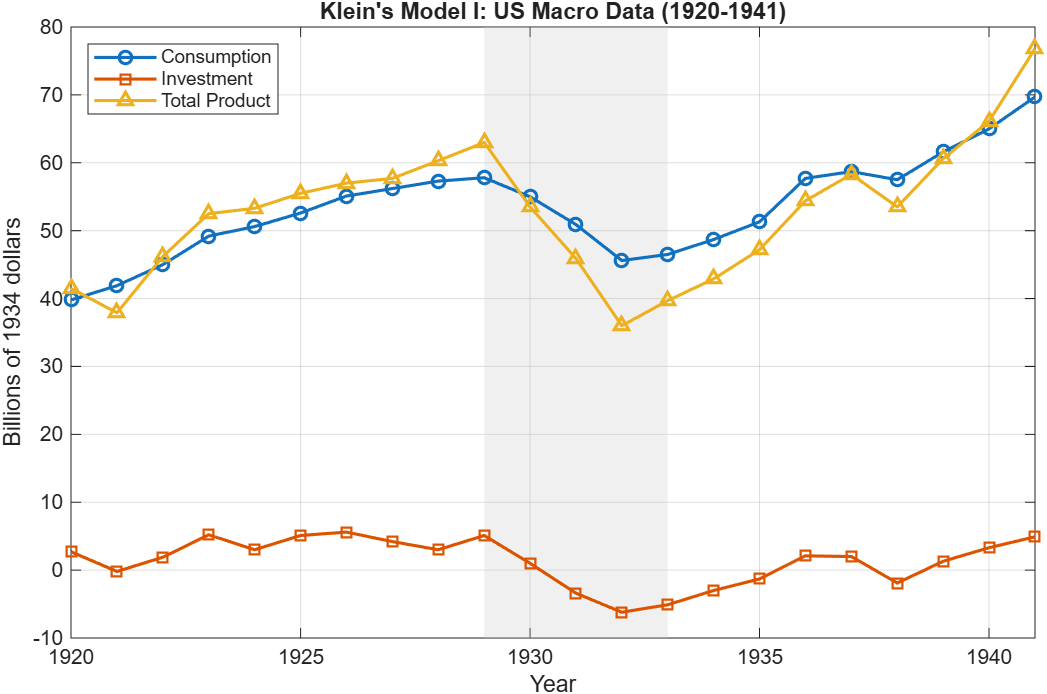
The collapse in investment during 1929-1933 is visible, and so is the asymmetry: consumption fell modestly while investment went negative.

From Workfile to Estimation: CAPM in Five Lines

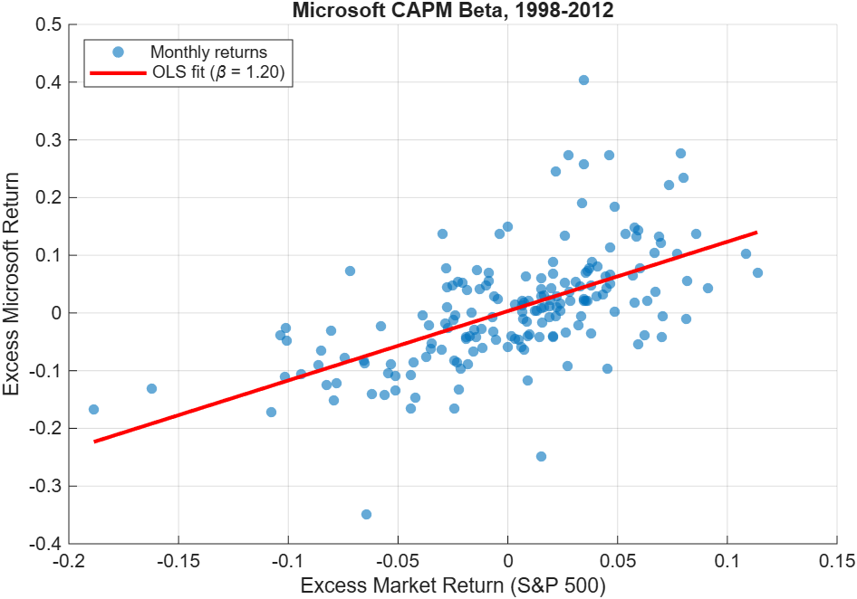
To show a complete load-to-estimation workflow, we switch to a second workfile: capm5.wf1, containing monthly stock returns for six firms plus the S&P 500 market portfolio and a risk-free rate (1998-2012).

The Capital Asset Pricing Model (CAPM) posits that a stock’s excess return is proportional to the market’s excess return, with the slope coefficient β measuring systematic risk.

% Load
  T = wfread("capm5.wf1", OutputType="timetable");

  % Compute excess returns
  T.ExcessMSFT = T.MSFT - T.RISKFREE;
  T.ExcessMKT  = T.MKT  - T.RISKFREE;

  % Estimate CAPM beta
  tbl = timetable2table(T, 'ConvertRowTimes', false);
  mdl = fitlm(tbl, 'ExcessMSFT ~ ExcessMKT');
  disp(mdl)

Results:

Linear regression model:
      ExcessMSFT ~ 1 + ExcessMKT

  Estimated Coefficients:
                     Estimate       SE        tStat       pValue
                     _________    ________    _______    __________
      (Intercept)    0.0032496    0.006036    0.53838      0.59098
      ExcessMKT        1.2018     0.12215     9.8389    1.63e-18

  R-squared: 0.352,  F-statistic vs. constant model: 96.8, p-value = 1.63e-18

Microsoft’s estimated β of 1.20 means its excess returns were more sensitive to market excess returns than a beta-one benchmark during this sample period. The R² of 0.352 shows that the single-factor model explains about 35% of the variation in Microsoft excess returns.

The Econometric Modeler app (Econometrics Toolbox) provides an interactive alternative. Load the timetable into the workspace, open the app with econometricModeler, and import from the workspace to explore, test, and fit models visually, then generate code when ready to automate.

What Else Can the Reader Handle?

For EViews 7+ binary workfiles, the reader can also extract:

• Groups: named collections of series, with member lists preserved
• Equations: estimated equation metadata (names and specifications)
• VARs: vector autoregression (VAR) model metadata
• Tables and Graphs: detected by name (WF1 table and graph cell data are not parsed)

The reader also supports the newer JSON-based .wf2 format introduced in EViews 12, which provides full object detail for all types.

Summary

What	How
Load a workfile	wf = wfread(“data.wf1”)
Get a timetable	T = wfread(“data.wf1″, OutputType=”timetable”)
Check metadata	wf.Metadata.Frequency, .StartYear, .NumObs
Read descriptions	wf.Metadata.SeriesDescriptions.VARNAME
Observed vs derived	wf.Metadata.ObservedSeries, .DerivedSeries

The MATLAB Reader for EViews Workfile is open source and available on GitHub under a BSD-3-Clause license. It reads legacy .wf1 files and newer .wf2 files, with no EViews installation required. Basic reading requires MATLAB R2021a or later and no additional toolboxes. The CAPM example uses Statistics and Machine Learning Toolbox, and the visual modeling workflow uses Econometrics Toolbox.

Data used in this post from Hill, Griffiths, and Lim, Principles of Econometrics, 5th Edition companion site. Underlying data sourced from US Bureau of Economic Analysis, Bureau of Labor Statistics, Wharton Research Data Services, and FRED.