Contour and Infinities
In a recent post, I talked about an interesting edge case in the contour function. Today I'd like to talk about another one. This is how contour handles infinities.
Let's start with a simple example. Here I've got a 4x3 array of values.
[x,y] = meshgrid(4:7,4:6);
z = x+y;
contourf(x,y,z,'LevelList',[8 10 13])

I'll make things a little easier to follow by using a variation on the labelcontourvalues function that I used in the earlier post to label the values at the vertices.
type labelcontourvalues
labelcontourvalues(x,y,z)
function labelcontourvalues(x,y,z)
    for r=1:size(z,1)
        for c=1:size(z,2)
            v = z(r,c);
            if (v<-15 || v>45 || isnan(v))
                color = 'red';
            else
                color = [.5 .5 .5];
            end
            h = text(x(r,c),y(r,c),num2str(v));
            h.HorizontalAlignment = 'center';
            h.VerticalAlignment = 'middle';
            h.Color = color;
            h.FontSize = 10;
            h.Margin = eps;
        end
    end
    ax = gca;
    xr = ax.XAxis;
    xr.TickValues = unique(x(:));
    xr.TickLabelFormat = 'X=%g';
    xr.FontSize = 6;
    yr = ax.YAxis;
    yr.TickValues = unique(y(:));
    yr.TickLabelFormat = 'Y=%g';
    yr.FontSize = 6;
    grid(ax,'on')
end
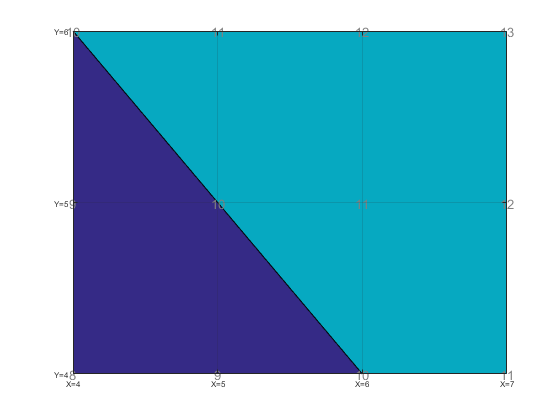
In this picture, the blue represents values between 8 and 10, while the teal represents values between 10 and 13. You can't see them, but yellow would represent values about 13, while a hole would represent values below 8.
If we stick an infinity at 6,5 we get the following.
tmp_z = z;
tmp_z(2,3) = inf;
contourf(x,y,tmp_z,'LevelList',[8 10 13])
labelcontourvalues(x,y,tmp_z)
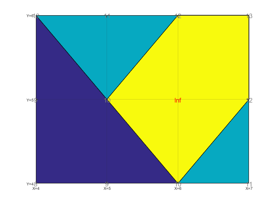
Does that seem right? It seems wrong, because the yellow region is touching the blue region. Shouldn't there be a teal region in between them?
What happens if we use a large, but finite value instead?
tmp_z = z;
tmp_z(2,3) = 50;
contourf(x,y,tmp_z,'LevelList',[8 10 13])
labelcontourvalues(x,y,tmp_z)
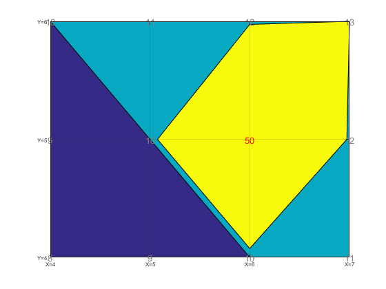
You can see that the value of 50 is surrounded by a yellow area (> 13) which reaches almost all the way to the neighboring values. On the side towards the blue region, the teal is just a thin sliver. In fact, it's 7.5% percent of the distance from the edge of the blue region to the vertex with value 50. That's because we're doing linear interpolation, and
$$(13-10)/(50-10)$$
is 7.5%.
If that 50 is replaced by infinity the denominator in that equation becomes infinitely large. Therefore, the width of the teal region shrinks to be infinitely thin.
Now lets do the same exercise with a negative infinity.
tmp_z = z;
tmp_z(2,2) = -inf;
contourf(x,y,tmp_z,'LevelList',[8 10 13])
labelcontourvalues(x,y,tmp_z)
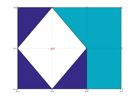
Does that seem right to you? We see that the area around the negative infinity is surrounded by a hole (< 8). That seems correct. By why did the blue region at X=6 move up to Y=5? We can see the reason if we use a large, but finite negative value instead.
tmp_z = z;
tmp_z(2,2) = -20;
contourf(x,y,tmp_z,'LevelList',[8 10 13])
labelcontourvalues(x,y,tmp_z)
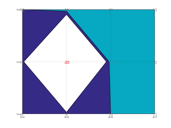
You can see that the blue region is actually going up and around the hole. It’s just that the negative infinity made that blue region infinitely narrow.
OK, now for the fun edge case. What happens when a positive infinity and a negative infinity are neighbors? I think that it should look something like this.
tmp_z = z;
tmp_z(2,2) = -inf;
tmp_z(2,3) = inf;
contourf(x,y,tmp_z,'LevelList',[8 10 13])
labelcontourvalues(x,y,tmp_z)
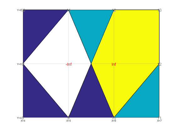
Do you agree?
The idea is that there’s actually an infinitely thin blue border going around the top of the hole, and an infinitely thin teal border sneaking between the blue and the yellow.
Here’s the non-infinite version for comparison:
tmp_z = z;
tmp_z(2,2) = -20;
tmp_z(2,3) = 50;
contourf(x,y,tmp_z,'LevelList',[8 10 13])
labelcontourvalues(x,y,tmp_z)
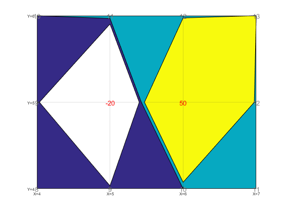
Although, if contour used a higher order interpolation function (as we talked about in this post), then it might look more like this:
[x2,y2] = meshgrid(linspace(4,7,150), ...
                   linspace(4,6,150));
z2 = interp2(x,y,tmp_z, x2,y2, 'cubic');
contourf(x2,y2,z2,'LevelList',[8 10 13])
labelcontourvalues(x,y,tmp_z)
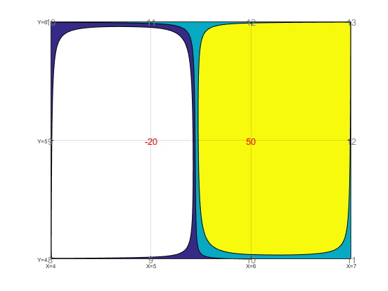
As you can see, the curves cross the grid lines in the same place. It's just that contour's default interpolation has cut straight across the center of each of the 2x2 squares, while the higher order interpolation has gone way around the side away from the large values.
So that's positive and negative infinity. What about NaN? This one's a little different because a NaN there's no way to define which side of a contour level a NaN is on. For this reason, the portion of a 2x2 square which is closest to a NaN is simply left empty.
tmp_z = z;
tmp_z(2,3) = nan;
contourf(x,y,tmp_z,'LevelList',[8 10 13])
labelcontourvalues(x,y,tmp_z)
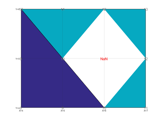
The portion that's not empty, continues to to linear interpolation, as we can see if we add more contour levels.
contourf(x,y,tmp_z,'LevelList',[8 10 11 12.5 13])
labelcontourvalues(x,y,tmp_z)
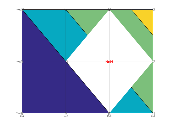
Notice that there isn't a black line around the white hole. That's because this area is undefined, rather than being defined by a contour line.
It might be nice if the contour functions would do something different near NaNs. The problem is that there isn't one "right answer" that works well in all situations. You really need to choose a method that's appropriate for your situation. That means that we would have to add a bunch of options to the contour functions to control this, but those options would be useless for most users of contour.
Luckily there are plenty of good MATLAB tools which can be used with the contour functions to control how NaNs are handled. One of my favorites is John D'Errico's inpaint_nans function, which is available on the File Exchange. It provides a number of options. The default is fine for this case, where the data is very smooth, ...
tmp_z2 = inpaint_nans(tmp_z);
contourf(x,y,tmp_z2,'LevelList',[8 10 11 12.5 13])
labelcontourvalues(x,y,tmp_z2)
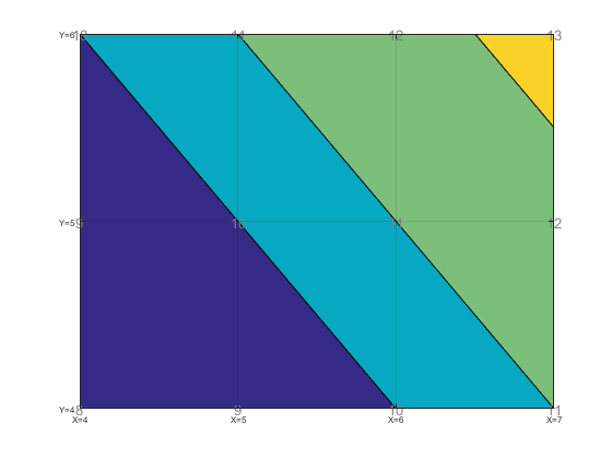
... but you might need to try one of the other options if you have several NaNs near each other, or data which has sharp gradients.
And, of course, you can combine something like inpaint_nans with the interp2 I used earlier to create a very powerful contouring workflow.
- Category:
- Geometry


