
NASA’s Artemis II mission and MATLAB
I was born in 1977. This was five years after the last crewed moon flight and so whilst I grew up hearing about the moon landings, I never experienced them. On April 2nd this year, that changed when Artemis II successfully launched from NASA's Kennedy Space Center.
In the 5+ years I've been at MathWorks, I've learned that whenever something really cool happens in science and engineering there is a good chance that the scientists and engineers involved used our tools. Artemis II is no different.
Designing the Space Launch System
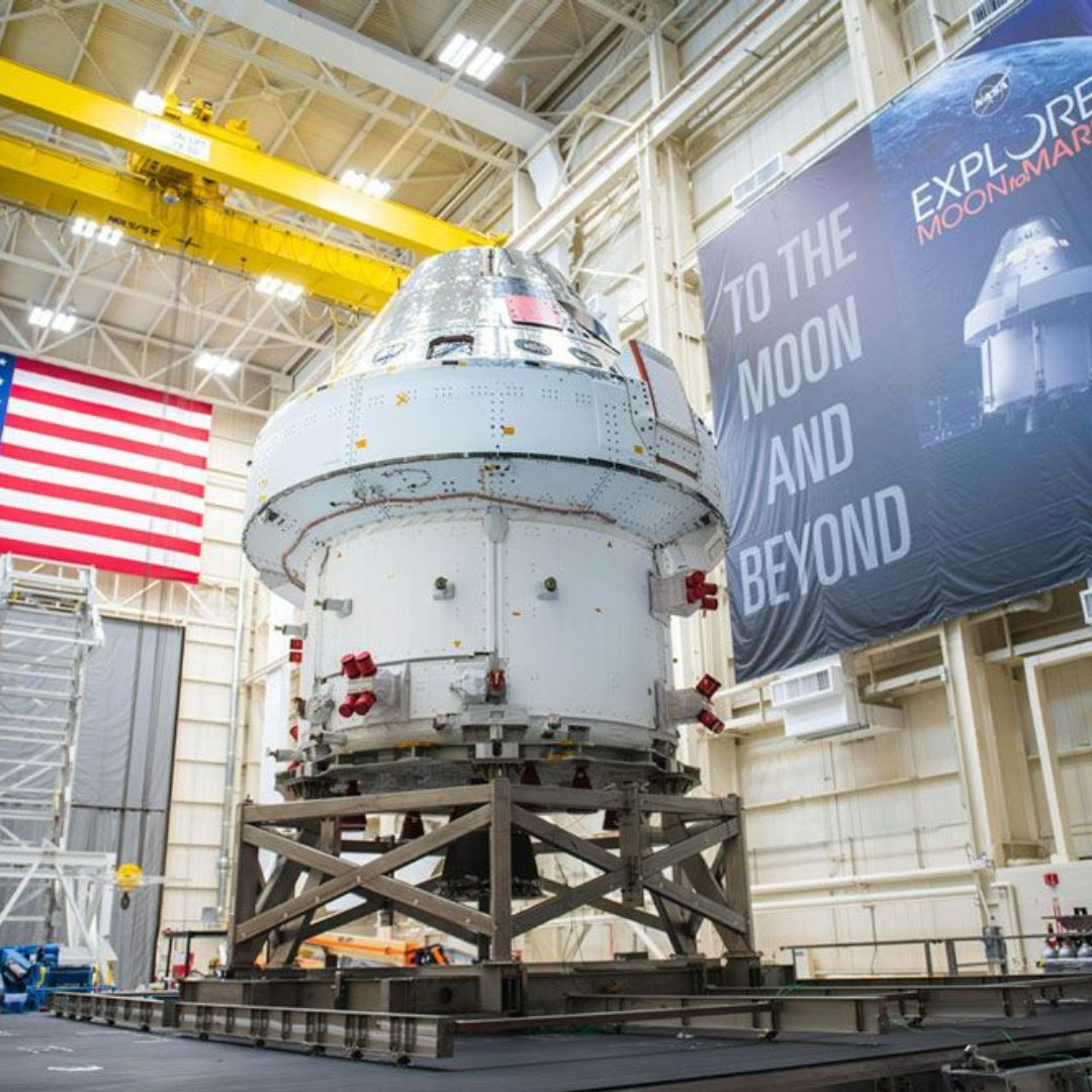
The crew on board are in the Orion Spacecraft (below) sitting atop the Space Launch System (SLS). The power system includes batteries, solar panels, computers, wires, and connections.
In designing the SLS, the engineers and scientists at NASA created a software model to simulate the mission-critical algorithms. Simulink, Simscape, and MATLAB are used throughout the Model-Based Design process to build an executable model. More details about NASA's Artemis Program and how MATLAB and Simulink are used can be found here.
Learning more about Artemis II's communications system
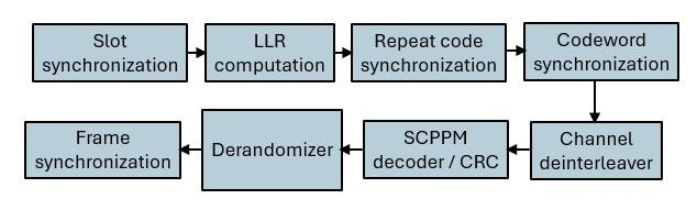
I searched LinkedIn to see what else other MathWorkers were saying about this mission and discovered that Artemis II uses an advanced optical communications system to send video, telemetry, and other data back to Earth. The system is based on a standard issued by the Consultative Committee for Space Data Systems (CCSDS), and uses a high photon efficiency (HPE) architecture that excels when power is at a premium.
It turns out that you can model this link in MATLAB! Check out this link for more details. If you are new to optical communications, this is a great example to learn some foundational principles of optical channel modeling and receiver design.
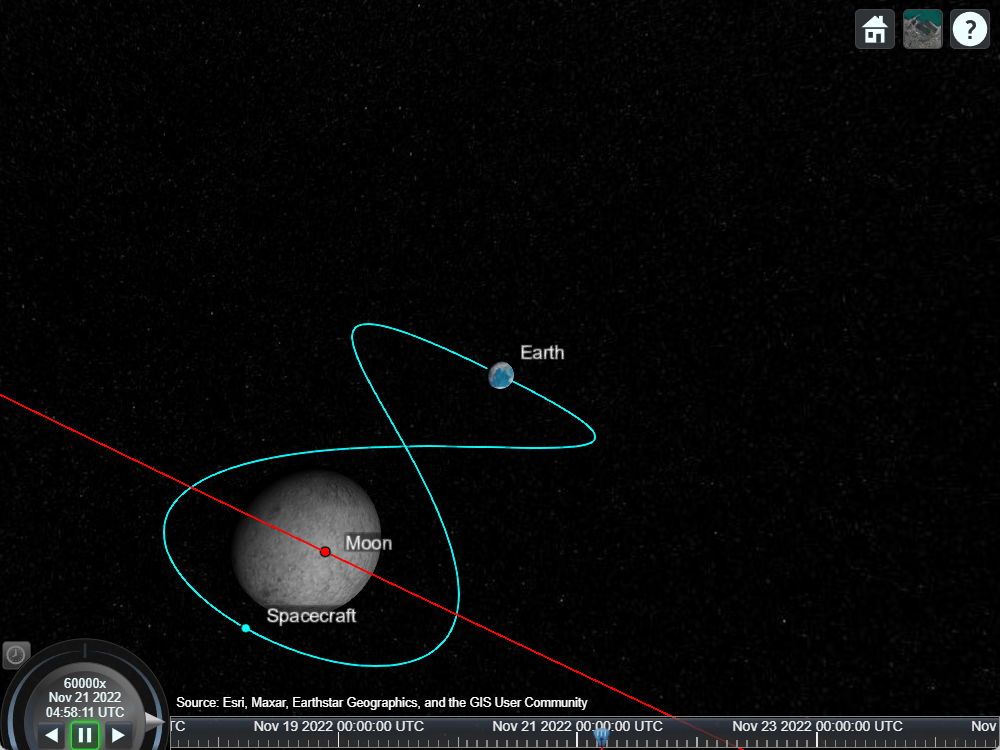
Visualize Artemis II's orbit trajectory using MATLAB's Satellite Scenario Viewer.
Although the four astronauts will not be landing, they will be flying around the far side of the moon before using the Moon's gravity to swing back to Earth. My colleague, Eric Hillsberg, modeled the mission using MATLAB's Satellite Scenario Viewer. In the video: the complete trajectory broken into phases: LEO insertion (Δv = 2,279 m/s), HEO transfer (Δv = 360 m/s), trans-lunar injection, lunar flyby at 6,999 km perilune, and return to Earth.


评论
要发表评论,请点击 此处 登录到您的 MathWorks 帐户或创建一个新帐户。